Calculating Dataset Information
These recipes demonstrate methods of calculating quantities in a simulation, either for later visualization or for understanding properties of fluids and particles in the simulation.
Average Field Value
This recipe is a very simple method of calculating the global average of a given field, as weighted by another field. See Processing Objects: Derived Quantities for more information.
import yt

ds = yt.load("IsolatedGalaxy/galaxy0030/galaxy0030")  # load data

field = ("gas", "temperature")  # The field to average
weight = ("gas", "mass")  # The weight for the average

ad = ds.all_data()  # This is a region describing the entire box,
# but note it doesn't read anything in yet!

# We now use our 'quantities' call to get the average quantity
average_value = ad.quantities.weighted_average_quantity(field, weight)

print(
    "Average %s (weighted by %s) is %0.3e %s"
    % (field[1], weight[1], average_value, average_value.units)
)
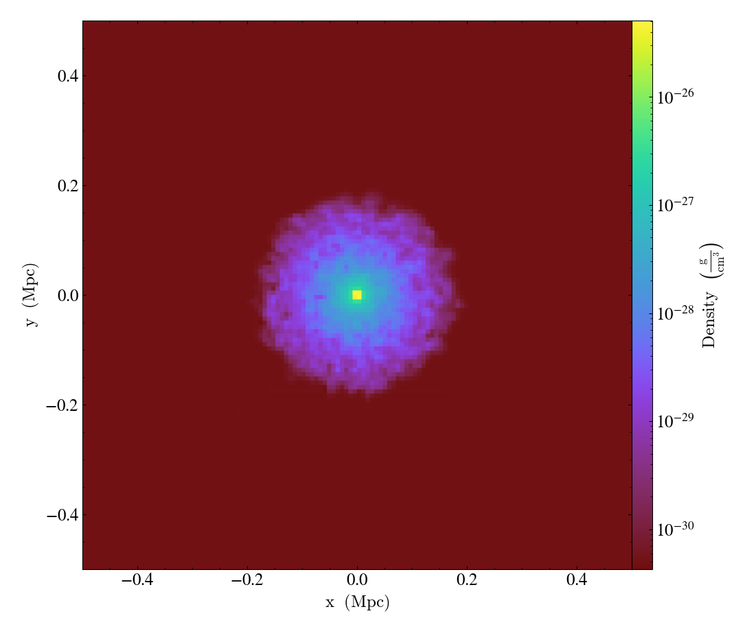
Mass Enclosed in a Sphere
This recipe constructs a sphere and then sums the total mass in particles and fluids in the sphere. See Available Objects and Processing Objects: Derived Quantities for more information.
import yt

# Load the dataset.
ds = yt.load("Enzo_64/DD0029/data0029")

# Create a 1 Mpc radius sphere, centered on the max density.
sp = ds.sphere("max", (1.0, "Mpc"))

# Use the total_quantity derived quantity to sum up the
# values of the mass and particle_mass fields
# within the sphere.
baryon_mass, particle_mass = sp.quantities.total_quantity(
    [("gas", "mass"), ("all", "particle_mass")]
)

print(
    "Total mass in sphere is %0.3e Msun (gas = %0.3e Msun, particles = %0.3e Msun)"
    % (
        (baryon_mass + particle_mass).in_units("Msun"),
        baryon_mass.in_units("Msun"),
        particle_mass.in_units("Msun"),
    )
)
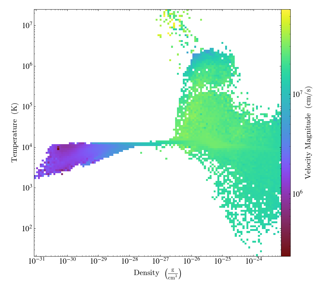
Global Phase Plot
This is a simple recipe to show how to open a dataset and then plot a couple global phase diagrams, save them, and quit. See 2D Phase Plots for more information.
import yt

# load the dataset
ds = yt.load("IsolatedGalaxy/galaxy0030/galaxy0030")

# This is an object that describes the entire box
ad = ds.all_data()

# We plot the average velocity magnitude (mass-weighted) in our object
# as a function of density and temperature
plot = yt.PhasePlot(
    ad, ("gas", "density"), ("gas", "temperature"), ("gas", "velocity_magnitude")
)

# save the plot
plot.save()
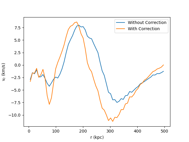
Radial Velocity Profile
This recipe demonstrates how to subtract off a bulk velocity on a sphere before calculating the radial velocity within that sphere. See 1D Profile Plots for more information on creating profiles and Field Parameters for an explanation of how the bulk velocity is provided to the radial velocity field function.
import matplotlib.pyplot as plt

import yt

ds = yt.load("GasSloshing/sloshing_nomag2_hdf5_plt_cnt_0150")

# Get the first sphere
sp0 = ds.sphere(ds.domain_center, (500.0, "kpc"))

# Compute the bulk velocity from the cells in this sphere
bulk_vel = sp0.quantities.bulk_velocity()


# Get the second sphere
sp1 = ds.sphere(ds.domain_center, (500.0, "kpc"))

# Set the bulk velocity field parameter
sp1.set_field_parameter("bulk_velocity", bulk_vel)

# Radial profile without correction

rp0 = yt.create_profile(
    sp0,
    ("index", "radius"),
    ("gas", "radial_velocity"),
    units={("index", "radius"): "kpc"},
    logs={("index", "radius"): False},
)

# Radial profile with correction for bulk velocity

rp1 = yt.create_profile(
    sp1,
    ("index", "radius"),
    ("gas", "radial_velocity"),
    units={("index", "radius"): "kpc"},
    logs={("index", "radius"): False},
)

# Make a plot using matplotlib

fig = plt.figure()
ax = fig.add_subplot(111)

ax.plot(
    rp0.x.value,
    rp0["gas", "radial_velocity"].in_units("km/s").value,
    rp1.x.value,
    rp1["gas", "radial_velocity"].in_units("km/s").value,
)

ax.set_xlabel(r"$\mathrm{r\ (kpc)}$")
ax.set_ylabel(r"$\mathrm{v_r\ (km/s)}$")
ax.legend(["Without Correction", "With Correction"])

fig.savefig(f"{ds}_profiles.png")
Simulation Analysis
This uses DatasetSeries to
calculate the extrema of a series of outputs, whose names it guesses in
advance. This will run in parallel and take advantage of multiple MPI tasks.
See Parallel Computation With yt and Time Series Analysis for more
information.
import yt

yt.enable_parallelism()

# Enable parallelism in the script (assuming it was called with
# `mpirun -np <n_procs>` )
yt.enable_parallelism()

# By using wildcards such as ? and * with the load command, we can load up a
# Time Series containing all of these datasets simultaneously.
ts = yt.load("enzo_tiny_cosmology/DD????/DD????")

# Calculate and store density extrema for all datasets along with redshift
# in a data dictionary with entries as tuples

# Create an empty dictionary
data = {}

# Iterate through each dataset in the Time Series (using piter allows it
# to happen in parallel automatically across available processors)
for ds in ts.piter():
    ad = ds.all_data()
    extrema = ad.quantities.extrema(("gas", "density"))

    # Fill the dictionary with extrema and redshift information for each dataset
    data[ds.basename] = (extrema, ds.current_redshift)

# Sort dict by keys
data = {k: v for k, v in sorted(data.items())}

# Print out all the values we calculated.
print("Dataset      Redshift        Density Min      Density Max")
print("---------------------------------------------------------")
for key, val in data.items():
    print(
        "%s       %05.3f          %5.3g g/cm^3   %5.3g g/cm^3"
        % (key, val[1], val[0][0], val[0][1])
    )
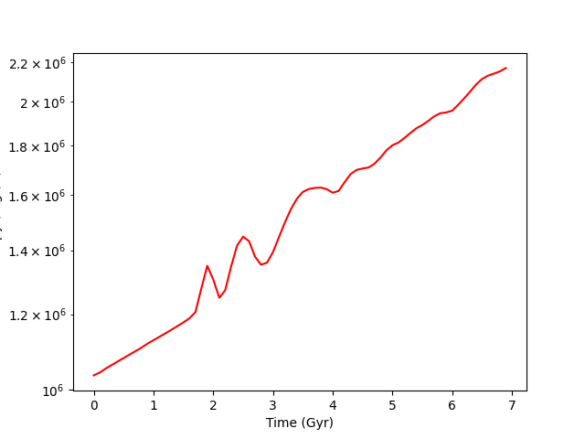
Time Series Analysis
This recipe shows how to calculate a number of quantities on a set of parameter
files. Note that it is parallel aware, and that if you only wanted to run in
serial the operation for pf in ts: would also have worked identically.
See Parallel Computation With yt and Time Series Analysis for more
information.
import matplotlib.pyplot as plt
import numpy as np

import yt

# Enable parallelism in the script (assuming it was called with
# `mpirun -np <n_procs>` )
yt.enable_parallelism()

# By using wildcards such as ? and * with the load command, we can load up a
# Time Series containing all of these datasets simultaneously.
# The "entropy" field that we will use below depends on the electron number
# density, which is not in these datasets by default, so we assume full
# ionization using the "default_species_fields" kwarg.
ts = yt.load(
    "GasSloshingLowRes/sloshing_low_res_hdf5_plt_cnt_0*",
    default_species_fields="ionized",
)

storage = {}

# By using the piter() function, we can iterate on every dataset in
# the TimeSeries object.  By using the storage keyword, we can populate
# a dictionary where the dataset is the key, and sto.result is the value
# for later use when the loop is complete.

# The serial equivalent of piter() here is just "for ds in ts:" .

for store, ds in ts.piter(storage=storage):
    # Create a sphere of radius 100 kpc at the center of the dataset volume
    sphere = ds.sphere("c", (100.0, "kpc"))
    # Calculate the entropy within that sphere
    entr = sphere["gas", "entropy"].sum()
    # Store the current time and sphere entropy for this dataset in our
    # storage dictionary as a tuple
    store.result = (ds.current_time.in_units("Gyr"), entr)

# Convert the storage dictionary values to a Nx2 array, so the can be easily
# plotted
arr = np.array(list(storage.values()))

# Plot up the results: time versus entropy
plt.semilogy(arr[:, 0], arr[:, 1], "r-")
plt.xlabel("Time (Gyr)")
plt.ylabel("Entropy (ergs/K)")
plt.savefig("time_versus_entropy.png")
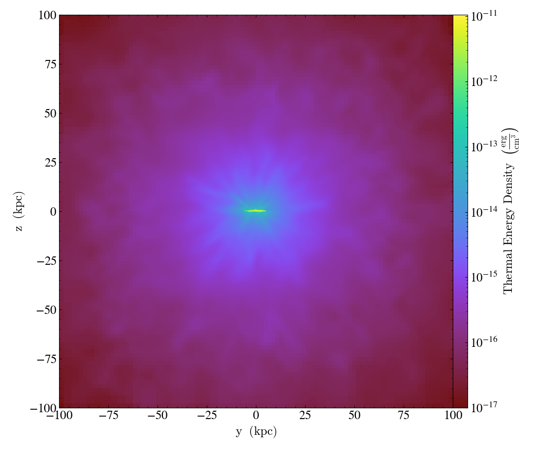
Simple Derived Fields
This recipe demonstrates how to create a simple derived field,
thermal_energy_density, and then generate a projection from it.
See Creating Derived Fields and Projection Plots for more
information.
import yt

# Load the dataset.
ds = yt.load("IsolatedGalaxy/galaxy0030/galaxy0030")

# You can create a derived field by manipulating any existing derived fields
# in any way you choose.  In this case, let's just make a simple one:
# thermal_energy_density = 3/2 nkT


# First create a function which yields your new derived field
def thermal_energy_dens(field, data):
    return (3 / 2) * data["gas", "number_density"] * data["gas", "kT"]


# Then add it to your dataset and define the units
ds.add_field(
    ("gas", "thermal_energy_density"),
    units="erg/cm**3",
    function=thermal_energy_dens,
    sampling_type="cell",
)

# It will now show up in your derived_field_list
for i in sorted(ds.derived_field_list):
    print(i)

# Let's use it to make a projection
ad = ds.all_data()
yt.ProjectionPlot(
    ds,
    "x",
    ("gas", "thermal_energy_density"),
    weight_field=("gas", "density"),
    width=(200, "kpc"),
).save()
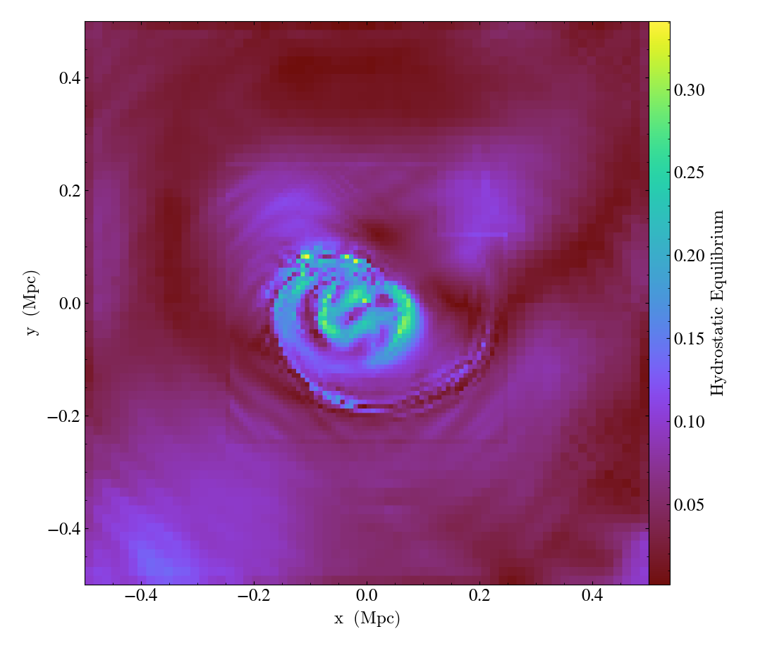
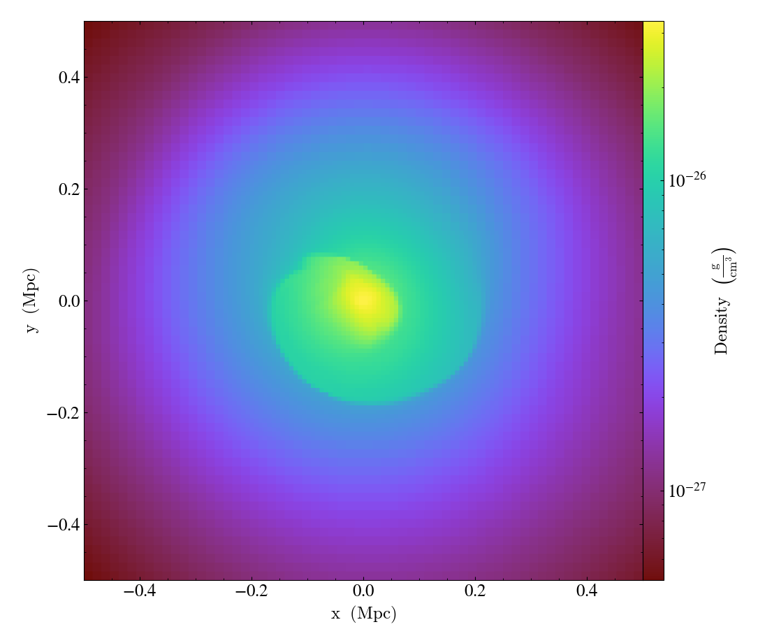
Complicated Derived Fields
This recipe demonstrates how to use the
add_gradient_fields() method
to generate gradient fields and use them in a more complex derived field.
import numpy as np

import yt

# Open a dataset from when there's a lot of sloshing going on.

ds = yt.load("GasSloshingLowRes/sloshing_low_res_hdf5_plt_cnt_0350")

# Define the components of the gravitational acceleration vector field by
# taking the gradient of the gravitational potential
grad_fields = ds.add_gradient_fields(("gas", "gravitational_potential"))

# We don't need to do the same for the pressure field because yt already
# has pressure gradient fields. Now, define the "degree of hydrostatic
# equilibrium" field.


def _hse(field, data):
    # Remember that g is the negative of the potential gradient
    gx = -data["gas", "density"] * data["gas", "gravitational_potential_gradient_x"]
    gy = -data["gas", "density"] * data["gas", "gravitational_potential_gradient_y"]
    gz = -data["gas", "density"] * data["gas", "gravitational_potential_gradient_z"]
    hx = data["gas", "pressure_gradient_x"] - gx
    hy = data["gas", "pressure_gradient_y"] - gy
    hz = data["gas", "pressure_gradient_z"] - gz
    h = np.sqrt((hx * hx + hy * hy + hz * hz) / (gx * gx + gy * gy + gz * gz))
    return h


ds.add_field(
    ("gas", "HSE"),
    function=_hse,
    units="",
    take_log=False,
    display_name="Hydrostatic Equilibrium",
    sampling_type="cell",
)

# The gradient operator requires periodic boundaries.  This dataset has
# open boundary conditions.
ds.force_periodicity()

# Take a slice through the center of the domain
slc = yt.SlicePlot(ds, 2, [("gas", "density"), ("gas", "HSE")], width=(1, "Mpc"))

slc.save("hse")
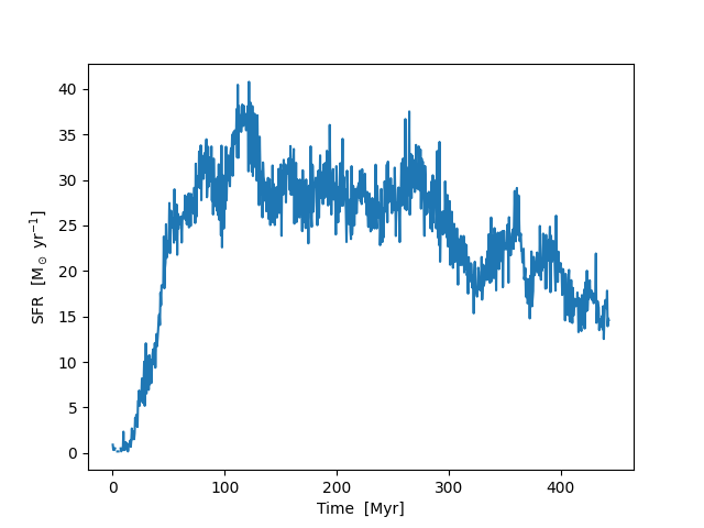
Using Particle Filters to Calculate Star Formation Rates
This recipe demonstrates how to use a particle filter to calculate the star formation rate in a galaxy evolution simulation. See Filtering Particle Fields for more information.
import numpy as np
from matplotlib import pyplot as plt

import yt
from yt.data_objects.particle_filters import add_particle_filter


def formed_star(pfilter, data):
    filter = data["all", "creation_time"] > 0
    return filter


add_particle_filter(
    "formed_star", function=formed_star, filtered_type="all", requires=["creation_time"]
)

filename = "IsolatedGalaxy/galaxy0030/galaxy0030"

ds = yt.load(filename)
ds.add_particle_filter("formed_star")
ad = ds.all_data()
masses = ad["formed_star", "particle_mass"].in_units("Msun")
formation_time = ad["formed_star", "creation_time"].in_units("yr")

time_range = [0, 5e8]  # years
n_bins = 1000
hist, bins = np.histogram(
    formation_time,
    bins=n_bins,
    range=time_range,
)
inds = np.digitize(formation_time, bins=bins)
time = (bins[:-1] + bins[1:]) / 2

sfr = np.array(
    [masses[inds == j + 1].sum() / (bins[j + 1] - bins[j]) for j in range(len(time))]
)
sfr[sfr == 0] = np.nan

plt.plot(time / 1e6, sfr)
plt.xlabel("Time  [Myr]")
plt.ylabel(r"SFR  [M$_\odot$ yr$^{-1}$]")
plt.savefig("filter_sfr.png")
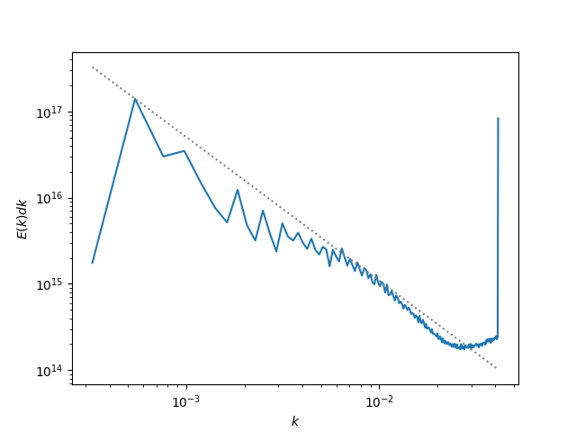
Making a Turbulent Kinetic Energy Power Spectrum
This recipe shows how to use yt to read data and put it on a uniform
grid to interface with the NumPy FFT routines and create a turbulent
kinetic energy power spectrum. (Note: the dataset used here is of low
resolution, so the turbulence is not very well-developed. The spike
at high wavenumbers is due to non-periodicity in the z-direction).
import matplotlib.pyplot as plt
import numpy as np

import yt

"""
Make a turbulent KE power spectrum.  Since we are stratified, we use
a rho**(1/3) scaling to the velocity to get something that would
look Kolmogorov (if the turbulence were fully developed).

Ultimately, we aim to compute:

                      1  ^      ^*
     E(k) = integral  -  V(k) . V(k) dS
                      2

             n                                               ^
where V = rho  U is the density-weighted velocity field, and V is the
FFT of V.

(Note: sometimes we normalize by 1/volume to get a spectral
energy density spectrum).


"""


def doit(ds):
    # a FFT operates on uniformly gridded data.  We'll use the yt
    # covering grid for this.

    max_level = ds.index.max_level

    ref = int(np.prod(ds.ref_factors[0:max_level]))

    low = ds.domain_left_edge
    dims = ds.domain_dimensions * ref

    nx, ny, nz = dims

    nindex_rho = 1.0 / 3.0

    Kk = np.zeros((nx // 2 + 1, ny // 2 + 1, nz // 2 + 1))

    for vel in [("gas", "velocity_x"), ("gas", "velocity_y"), ("gas", "velocity_z")]:
        Kk += 0.5 * fft_comp(
            ds, ("gas", "density"), vel, nindex_rho, max_level, low, dims
        )

    # wavenumbers
    L = (ds.domain_right_edge - ds.domain_left_edge).d

    kx = np.fft.rfftfreq(nx) * nx / L[0]
    ky = np.fft.rfftfreq(ny) * ny / L[1]
    kz = np.fft.rfftfreq(nz) * nz / L[2]

    # physical limits to the wavenumbers
    kmin = np.min(1.0 / L)
    kmax = np.min(0.5 * dims / L)

    kbins = np.arange(kmin, kmax, kmin)
    N = len(kbins)

    # bin the Fourier KE into radial kbins
    kx3d, ky3d, kz3d = np.meshgrid(kx, ky, kz, indexing="ij")
    k = np.sqrt(kx3d**2 + ky3d**2 + kz3d**2)

    whichbin = np.digitize(k.flat, kbins)
    ncount = np.bincount(whichbin)

    E_spectrum = np.zeros(len(ncount) - 1)

    for n in range(1, len(ncount)):
        E_spectrum[n - 1] = np.sum(Kk.flat[whichbin == n])

    k = 0.5 * (kbins[0 : N - 1] + kbins[1:N])
    E_spectrum = E_spectrum[1:N]

    index = np.argmax(E_spectrum)
    kmax = k[index]
    Emax = E_spectrum[index]

    plt.loglog(k, E_spectrum)
    plt.loglog(k, Emax * (k / kmax) ** (-5.0 / 3.0), ls=":", color="0.5")

    plt.xlabel(r"$k$")
    plt.ylabel(r"$E(k)dk$")

    plt.savefig("spectrum.png")


def fft_comp(ds, irho, iu, nindex_rho, level, low, delta):
    cube = ds.covering_grid(level, left_edge=low, dims=delta, fields=[irho, iu])

    rho = cube[irho].d
    u = cube[iu].d

    nx, ny, nz = rho.shape

    # do the FFTs -- note that since our data is real, there will be
    # too much information here.  fftn puts the positive freq terms in
    # the first half of the axes -- that's what we keep.  Our
    # normalization has an '8' to account for this clipping to one
    # octant.
    ru = np.fft.fftn(rho**nindex_rho * u)[
        0 : nx // 2 + 1, 0 : ny // 2 + 1, 0 : nz // 2 + 1
    ]
    ru = 8.0 * ru / (nx * ny * nz)

    return np.abs(ru) ** 2


ds = yt.load("maestro_xrb_lores_23437")
doit(ds)
Downsampling an AMR Dataset
This recipe shows how to use the max_level attribute of a yt data
object to only select data up to a maximum AMR level.
import yt

ds = yt.load("IsolatedGalaxy/galaxy0030/galaxy0030")

# The maximum refinement level of this dataset is 8
print(ds.max_level)

# If we ask for *all* of the AMR data, we get back field
# values sampled at about 3.6 million AMR zones
ad = ds.all_data()
print(ad["gas", "density"].shape)

# Let's only sample data up to AMR level 2
ad.max_level = 2

# Now we only sample from about 200,000 zones
print(ad["gas", "density"].shape)

# Note that this includes data at level 2 that would
# normally be masked out. There aren't any "holes" in
# the downsampled AMR mesh, the volume still sums to
# the volume of the domain:
print(ad["gas", "volume"].sum())
print(ds.domain_width.prod())

# Now let's make a downsampled plot
plot = yt.SlicePlot(ds, "z", ("gas", "density"), data_source=ad)
plot.save("downsampled.png")