A Brief Demo of Volume Rendering

This shows a small amount of volume rendering. Really, just enough to get your feet wet!

import yt

ds = yt.load_sample("IsolatedGalaxy")

To create a volume rendering, we need a camera and a transfer function. We’ll use the ColorTransferFunction, which accepts (in log space) the minimum and maximum bounds of our transfer function. This means behavior for data outside these values is undefined.

We then add on “layers” like an onion. This function can accept a width (here specified) in data units, and also a color map. Here we add on four layers.

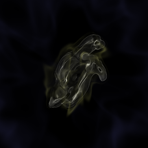
Finally, we create a camera. The focal point is [0.5, 0.5, 0.5], the width is 20 kpc (including front-to-back integration) and we specify a transfer function. Once we’ve done that, we call show to actually cast our rays and display them inline.

sc = yt.create_scene(ds)

sc.camera.set_width(ds.quan(20, "kpc"))

source = sc.sources["source_00"]

tf = yt.ColorTransferFunction((-28, -24))
tf.add_layers(4, w=0.01)

source.set_transfer_function(tf)

sc.show()

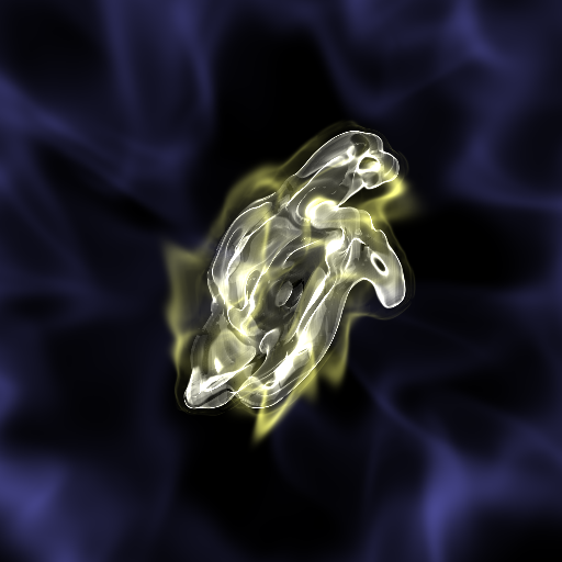
If we want to apply a clipping, we can specify the sigma_clip. This will clip the upper bounds to this value times the standard deviation of the values in the image array.

sc.show(sigma_clip=4)

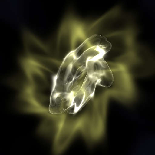
There are several other options we can specify. Note that here we have turned on the use of ghost zones, shortened the data interval for the transfer function, and widened our gaussian layers.

sc = yt.create_scene(ds)

sc.camera.set_width(ds.quan(20, "kpc"))

source = sc.sources["source_00"]

source.field = "density"

tf = yt.ColorTransferFunction((-28, -25))
tf.add_layers(4, w=0.03)

source.transfer_function = tf

sc.show(sigma_clip=4.0)