Loading Data via Functions

One of the things that yt provides is the notion of “derived fields.” These are fields that exist only in memory, and are defined by a functional form, typically transforming other fields. Starting with version 4.1 of yt, however, we have made it much, much easier to define so-called “on-disk” fields through their functional forms, akin to how derived fields are generated. At present, this is only available for grid-based frontends. Extension to other types is anticipated in future versions of yt.

What this means is that if you have a way to grab data – at any resolution – but don’t want to either load it into memory in advance or write a complete “frontend”, you can just write some functions and use those to construct a fully-functional dataset using the existing load_amr_grids and load_uniform_grid functions, supplying functions instead of arrays.

There are a few immediate use cases that can be seen for this:

• Data is accessible through another library, for instance if a library exists that reads subsets of data (or regularizes that data to given regions) or if you are calling yt from an in situ analysis library

• Data can be remotely accessed on-demand

• You have a straightforward data format for which a frontend does not exist

• All of the data can be generated through an analytical definition

The last one is what we’ll use to demonstrate this. Let’s imagine that I had a grid structure that I wanted to explore, but I wanted all of my data to be generated through functions that were exclusively dependent on the spatial position.

import matplotlib.pyplot as plt
import numpy as np

import yt

The example we’ve cooked up is going to be a bit silly, and we’ll demonstrate it a little bit with one and two dimensional setups before getting into the full yt demonstration. (If you have ideas for a better one, please do suggest them!) We’ll start with some overlapping trigonometric functions, which we’ll attenuate by their distance from the center.

So we’ll set up some coefficients for different periods of the functions (the coefficients variable) and we’ll sum up those functions. The next thing we’ll do, so that we have some global attenuation we can see, is use a Gaussian function centered at the center of our domain.

x = np.mgrid[0.0:1.0:512j]
coefficients = (100, 50, 30, 10)
y = sum(c * np.sin(2 ** (2 + i) * (x * np.pi * 2)) for i, c in enumerate(coefficients))
atten = np.exp(-20 * (1.1 * (x - 0.5)) ** 2)

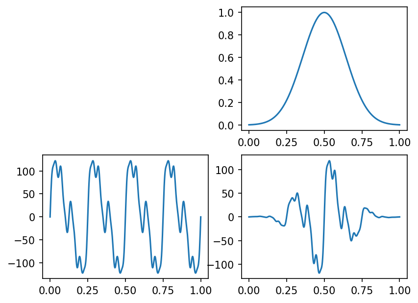
Now let’s plot it! The top right is the attenuation, bottom left is the base sum of trig functions, and then the bottom right is the product.

fig, ((ax1, ax2), (ax3, ax4)) = plt.subplots(2, 2, dpi=150)
ax4.plot(x, y * atten)
ax2.plot(x, atten)
ax3.plot(x, y)
ax1.axis(False);

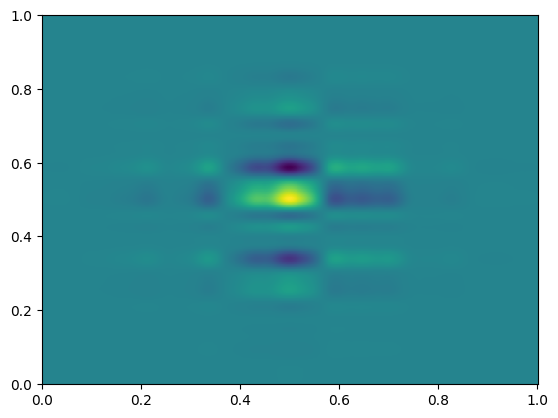
Well, that looks like it might have some structure at different scales! We should be able to use something like this to show sampling errors and so on in AMR, and it’ll have structure down to a reasonably high level of detail. Let’s briefly demonstrate in 2D before moving on to 3D, using similar functions. This is all basically the same as the previous cells, except we’re overlaying along a couple different dimensions.

x, y = np.mgrid[0.0:1.0:512j, 0.0:1.0:512j]

x_coefficients = (100, 50, 30, 10)
y_coefficients = (20, 90, 80, 30)

z = sum(
    c * np.sin(2 ** (1 + i) * (x * np.pi * 2 + 2**i))
    for i, c in enumerate(x_coefficients)
) * sum(
    c * np.sin(2 ** (1 + i) * (y * np.pi * 2 + 2**i))
    for i, c in enumerate(y_coefficients)
)
r = np.sqrt(((x - 0.5) ** 2) + ((y - 0.5) ** 2))
atten = np.exp(-20 * (1.1 * r**2))

plt.pcolormesh(x, y, z * atten)

<matplotlib.collections.QuadMesh at 0x7f671ec8d090>

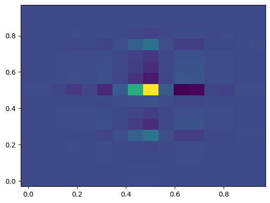
This is an image of the full dataset, but what happens if we coarsely sample, as we would in AMR simulations? We can stride along the axes (let’s say, every 32nd point) to get an idea of what that looks like.

plt.pcolormesh(x[::32, ::32], y[::32, ::32], (z * atten)[::32, ::32])

<matplotlib.collections.QuadMesh at 0x7f672153cb10>

For moving to 3D, I’m going to add on some higher-frequency modes, which I’ll also amplify a bit more. We’ll use the standard attenuation (although a directionally-dependent attenuation would be nice, wouldn’t it?)

And this time, we’ll write them into a special function. This is the function we’ll use to supply to our load_amr_grids function – it has different arguments than a derived field; because it is assumed to always return three-dimensional data, it accepts a proper grid object (which may have spatial or other attributes) and it also receives the field name.

Using this, we will compute the cell-centers for all of the cells in the grid, and use them to compute our overlapping functions and apply the attenuation. In doing so, we should be able to see structure at different levels. This is the same way you would write a function that loaded a file from disk, or received over HTTP, or used a library to read data; by having access to the grid and the field name, it should be completely determinative of how to access the data.

x_coefficients = (100, 50, 30, 10, 20)
y_coefficients = (20, 90, 80, 30, 30)
z_coefficients = (50, 10, 90, 40, 40)


def my_function(grid, field_name):
    # We want N points from the cell-center to the cell-center on the other side
    x, y, z = (
        np.linspace(
            grid.LeftEdge[i] + grid.dds[i] / 2,
            grid.RightEdge[i] - grid.dds[i] / 2,
            grid.ActiveDimensions[i],
        )
        for i in (0, 1, 2)
    )
    r = np.sqrt(
        ((x.d - 0.5) ** 2)[:, None, None]
        + ((y.d - 0.5) ** 2)[None, :, None]
        + ((z.d - 0.5) ** 2)[None, None, :]
    )
    atten = np.exp(-20 * (1.1 * r**2))
    xv = sum(
        c * np.sin(2 ** (1 + i) * (x.d * np.pi * 2))
        for i, c in enumerate(x_coefficients)
    )
    yv = sum(
        c * np.sin(2 ** (1 + i) * (y.d * np.pi * 2))
        for i, c in enumerate(y_coefficients)
    )
    zv = sum(
        c * np.sin(2 ** (1 + i) * (z.d * np.pi * 2))
        for i, c in enumerate(z_coefficients)
    )
    return atten * (xv[:, None, None] * yv[None, :, None] * zv[None, None, :])

We’ll use a standard grid hierarchy – which is used internally in yt testing – and fill it up with a single field that provides this function rather than any arrays. We’ll then use load_amr_grids to read it; note that we’re not creating any arrays ahead of time.

from yt.testing import _amr_grid_index

grid_data = []
for level, le, re, dims in _amr_grid_index:
    grid_data.append(
        {
            "level": level,
            "left_edge": le,
            "right_edge": re,
            "dimensions": dims,
            "density": my_function,
        }
    )
ds = yt.load_amr_grids(
    grid_data, [32, 32, 32], bbox=np.array([[0.0, 1.0], [0.0, 1.0], [0.0, 1.0]])
)

And finally, we’ll demonstrate it with a slice along the y axis.

p = ds.r[:, 0.5, :].plot("density").set_log("density", False)

And with a quick zoom, we can see that the structure is indeed present and subject to the sampling effects we discussed earlier.

p.zoom(4)