Plot Modifications: Overplotting Contours, Velocities, Particles, and More

Adding callbacks to plots

After a plot is generated using the standard tools (e.g. SlicePlot, ProjectionPlot, etc.), it can be annotated with any number of callbacks before being saved to disk. These callbacks can modify the plots by adding lines, text, markers, streamlines, velocity vectors, contours, and more.

Callbacks can be applied to plots created with SlicePlot, ProjectionPlot, AxisAlignedSlicePlot, AxisAlignedProjectionPlot, OffAxisSlicePlot, or OffAxisProjectionPlot, by calling one of the annotate_ methods that hang off of the plot object. The annotate_ methods are dynamically generated based on the list of available callbacks. For example:

slc = SlicePlot(ds, "x", ("gas", "density"))
slc.annotate_title("This is a Density plot")

would add the TitleCallback() to the plot object. All of the callbacks listed below are available via similar annotate_ functions.

To clear one or more annotations from an existing plot, see the clear_annotations function.

For a brief demonstration of a few of these callbacks in action together, see the cookbook recipe: Annotating Plots to Include Lines, Text, Shapes, etc..

Also note that new annotate_ methods can be defined without modifying yt’s source code, see Extending annotations methods.

Coordinate Systems in Callbacks

Many of the callbacks (e.g. TextLabelCallback) are specified to occur at user-defined coordinate locations (like where to place a marker or text on the plot). There are several different coordinate systems used to identify these locations. These coordinate systems can be specified with the coord_system keyword in the relevant callback, which is by default set to data. The valid coordinate systems are:

data – the 3D dataset coordinates

plot – the 2D coordinates defined by the actual plot limits

axis – the MPL axis coordinates: (0,0) is lower left; (1,1) is upper right

figure – the MPL figure coordinates: (0,0) is lower left, (1,1) is upper right

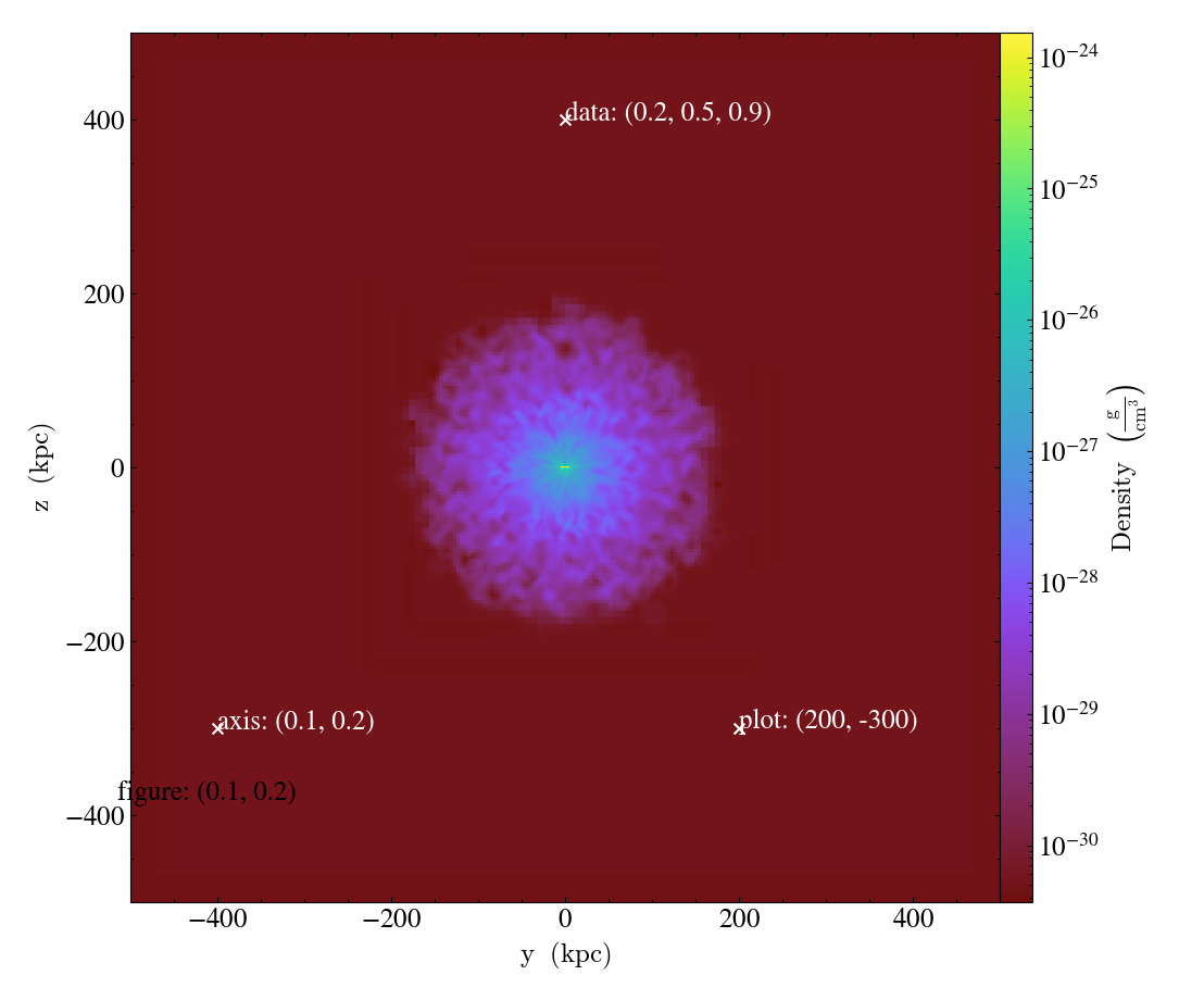
Here we will demonstrate these different coordinate systems for an projection of the x-plane (i.e. with axes in the y and z directions):

import yt

ds = yt.load("IsolatedGalaxy/galaxy0030/galaxy0030")
s = yt.SlicePlot(ds, "x", ("gas", "density"))
s.set_axes_unit("kpc")

# Plot marker and text in data coords
s.annotate_marker((0.2, 0.5, 0.9), coord_system="data")
s.annotate_text((0.2, 0.5, 0.9), "data: (0.2, 0.5, 0.9)", coord_system="data")

# Plot marker and text in plot coords
s.annotate_marker((200, -300), coord_system="plot")
s.annotate_text((200, -300), "plot: (200, -300)", coord_system="plot")

# Plot marker and text in axis coords
s.annotate_marker((0.1, 0.2), coord_system="axis")
s.annotate_text((0.1, 0.2), "axis: (0.1, 0.2)", coord_system="axis")

# Plot marker and text in figure coords
# N.B. marker will not render outside of axis bounds
s.annotate_marker((0.1, 0.2), coord_system="figure", color="black")
s.annotate_text(
    (0.1, 0.2),
    "figure: (0.1, 0.2)",
    coord_system="figure",
    text_args={"color": "black"},
)
s.save()

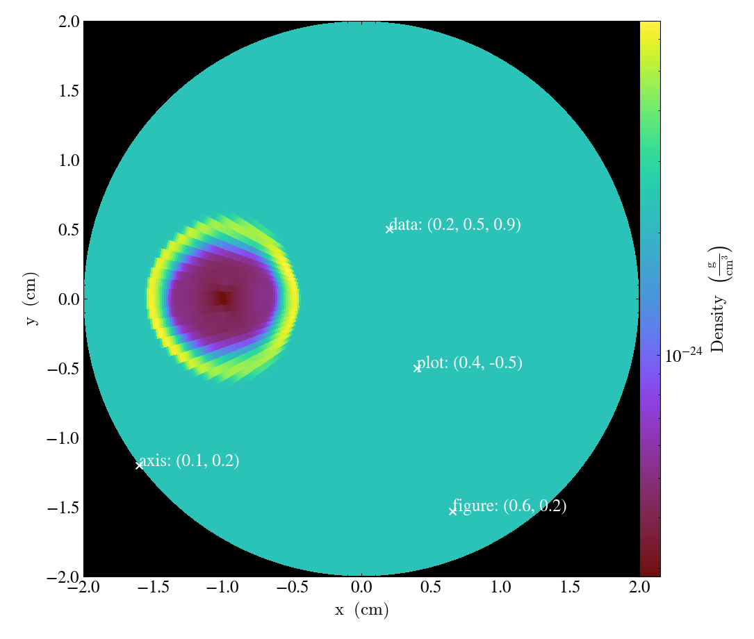
Note that for non-cartesian geometries and coord_system="data", the coordinates are still interpreted in the corresponding cartesian system. For instance using a polar dataset from AMRVAC :

import yt

ds = yt.load("amrvac/bw_polar_2D0000.dat")
s = yt.plot_2d(ds, ("gas", "density"))
s.set_background_color("density", "black")

# Plot marker and text in data coords
s.annotate_marker((0.2, 0.5, 0.9), coord_system="data")
s.annotate_text((0.2, 0.5, 0.9), "data: (0.2, 0.5, 0.9)", coord_system="data")

# Plot marker and text in plot coords
s.annotate_marker((0.4, -0.5), coord_system="plot")
s.annotate_text((0.4, -0.5), "plot: (0.4, -0.5)", coord_system="plot")

# Plot marker and text in axis coords
s.annotate_marker((0.1, 0.2), coord_system="axis")
s.annotate_text((0.1, 0.2), "axis: (0.1, 0.2)", coord_system="axis")

# Plot marker and text in figure coords
# N.B. marker will not render outside of axis bounds
s.annotate_marker((0.6, 0.2), coord_system="figure")
s.annotate_text((0.6, 0.2), "figure: (0.6, 0.2)", coord_system="figure")
s.save()

Available Callbacks

The underlying functions are more thoroughly documented in Callback List.

Clear Callbacks (Some or All)

clear_annotations(index=None)

This function will clear previous annotations (callbacks) in the plot. If no index is provided, it will clear all annotations to the plot. If an index is provided, it will clear only the Nth annotation to the plot. Note that the index goes from 0..N, and you can specify the index of the last added annotation as -1.

(This is a proxy for clear_annotations().)

import yt

ds = yt.load("IsolatedGalaxy/galaxy0030/galaxy0030")
p = yt.SlicePlot(ds, "z", ("gas", "density"), center="c", width=(20, "kpc"))
p.annotate_scale()
p.annotate_timestamp()

# Oops, I didn't want any of that.
p.clear_annotations()
p.save()

List Currently Applied Callbacks

list_annotations()

This function will print a list of each of the currently applied callbacks together with their index. The index can be used with clear_annotations() function to remove a specific callback.

(This is a proxy for list_annotations().)

import yt

ds = yt.load("IsolatedGalaxy/galaxy0030/galaxy0030")
p = yt.SlicePlot(ds, "z", ("gas", "density"), center="c", width=(20, "kpc"))
p.annotate_scale()
p.annotate_timestamp()
p.list_annotations()

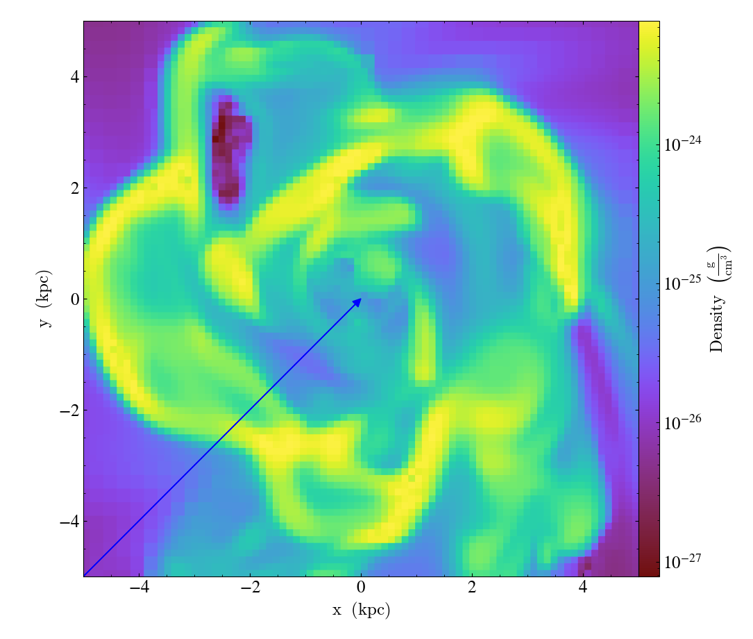
Overplot Arrow

annotate_arrow(self, pos, length=0.03, coord_system='data', **kwargs)

(This is a proxy for ArrowCallback.)

Overplot an arrow pointing at a position for highlighting a specific feature. Arrow points from lower left to the designated position with arrow length “length”.

import yt

ds = yt.load("IsolatedGalaxy/galaxy0030/galaxy0030")
slc = yt.SlicePlot(ds, "z", ("gas", "density"), width=(10, "kpc"), center="c")
slc.annotate_arrow((0.5, 0.5, 0.5), length=0.06, color="blue")
slc.save()

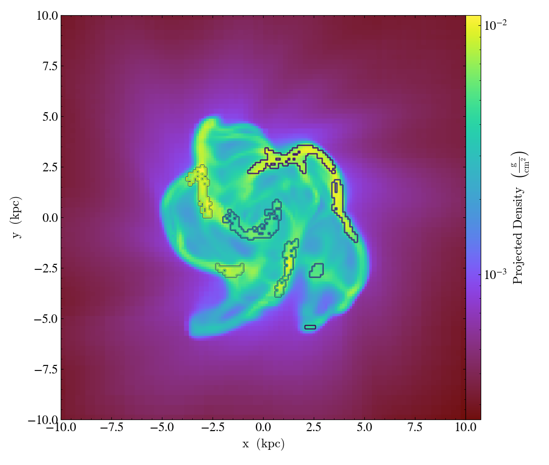
Clump Finder Callback

annotate_clumps(self, clumps, **kwargs)

(This is a proxy for ClumpContourCallback.)

Take a list of clumps and plot them as a set of contours.

import numpy as np

import yt
from yt.data_objects.level_sets.api import Clump, find_clumps

ds = yt.load("IsolatedGalaxy/galaxy0030/galaxy0030")
data_source = ds.disk([0.5, 0.5, 0.5], [0.0, 0.0, 1.0], (8.0, "kpc"), (1.0, "kpc"))

c_min = 10 ** np.floor(np.log10(data_source["gas", "density"]).min())
c_max = 10 ** np.floor(np.log10(data_source["gas", "density"]).max() + 1)

master_clump = Clump(data_source, ("gas", "density"))
master_clump.add_validator("min_cells", 20)

find_clumps(master_clump, c_min, c_max, 2.0)
leaf_clumps = master_clump.leaves

prj = yt.ProjectionPlot(ds, "z", ("gas", "density"), center="c", width=(20, "kpc"))
prj.annotate_clumps(leaf_clumps)
prj.save("clumps")

Overplot Contours

annotate_contour(self, field, levels=5, factor=4, take_log=False, clim=None, plot_args=None, label=False, text_args=None, data_source=None)

(This is a proxy for ContourCallback.)

Add contours in field to the plot. levels governs the number of contours generated, factor governs the number of points used in the interpolation, take_log governs how it is contoured and clim gives the (lower, upper) limits for contouring.

import yt

ds = yt.load("Enzo_64/DD0043/data0043")
s = yt.SlicePlot(ds, "x", ("gas", "density"), center="max")
s.annotate_contour(("gas", "temperature"))
s.save()

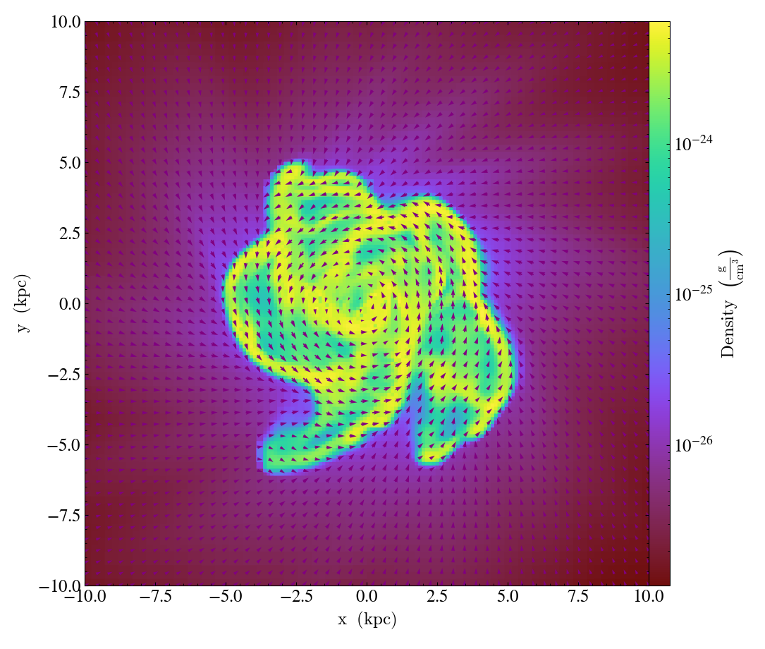
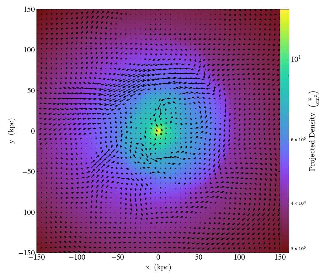
Overplot Quivers

Axis-Aligned Data Sources

annotate_quiver(self, field_x, field_y, field_c=None, *, factor=16, scale=None, scale_units=None, normalize=False, **kwargs)

(This is a proxy for QuiverCallback.)

Adds a ‘quiver’ plot to any plot, using the field_x and field_y from the associated data, skipping every factor pixels in the discretization. A third field, field_c, can be used as color; which is the counterpart of matplotlib.axes.Axes.quiver’s final positional argument C. scale is the data units per arrow length unit using scale_units. If normalize is True, the fields will be scaled by their local (in-plane) length, allowing morphological features to be more clearly seen for fields with substantial variation in field strength. All additional keyword arguments are passed down to matplotlib.Axes.axes.quiver.

Example using a constant color

import yt

ds = yt.load("IsolatedGalaxy/galaxy0030/galaxy0030")
p = yt.ProjectionPlot(
    ds,
    "z",
    ("gas", "density"),
    center=[0.5, 0.5, 0.5],
    weight_field="density",
    width=(20, "kpc"),
)
p.annotate_quiver(
   ("gas", "velocity_x"),
   ("gas", "velocity_y"),
   factor=16,
   color="purple",
)
p.save()

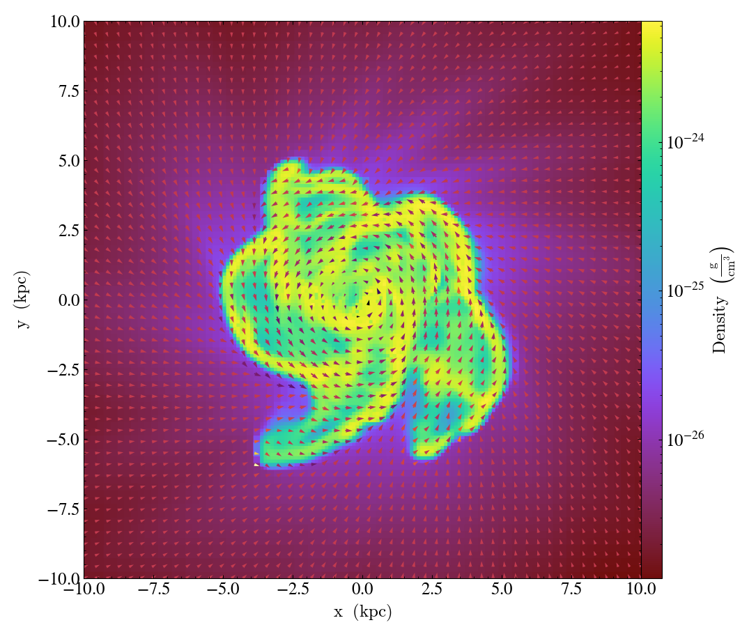
And now using a continuous colormap

import yt

ds = yt.load("IsolatedGalaxy/galaxy0030/galaxy0030")
p = yt.ProjectionPlot(
    ds,
    "z",
    ("gas", "density"),
    center=[0.5, 0.5, 0.5],
    weight_field="density",
    width=(20, "kpc"),
)
p.annotate_quiver(
   ("gas", "velocity_x"),
   ("gas", "velocity_y"),
   ("gas", "vorticity_z"),
   factor=16,
   cmap="inferno_r",
)
p.save()

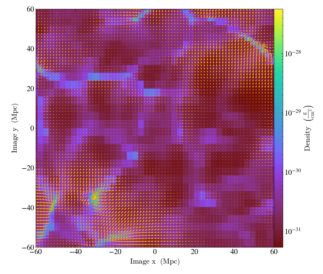
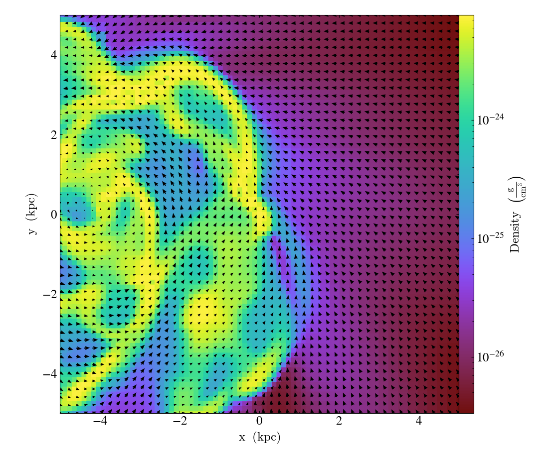
Off-Axis Data Sources

annotate_cquiver(self, field_x, field_y, field_c=None, *, factor=16, scale=None, scale_units=None, normalize=False, **kwargs)

(This is a proxy for CuttingQuiverCallback.)

Get a quiver plot on top of a cutting plane, using the field_x and field_y from the associated data, skipping every factor datapoints in the discretization. scale is the data units per arrow length unit using scale_units. If normalize is True, the fields will be scaled by their local (in-plane) length, allowing morphological features to be more clearly seen for fields with substantial variation in field strength. Additional arguments can be passed to the plot_args dictionary, see matplotlib.axes.Axes.quiver for more info.

import yt

ds = yt.load("Enzo_64/DD0043/data0043")
s = yt.OffAxisSlicePlot(ds, [1, 1, 0], [("gas", "density")], center="c")
s.annotate_cquiver(
    ("gas", "cutting_plane_velocity_x"),
    ("gas", "cutting_plane_velocity_y"),
    factor=10,
    color="orange",
)
s.zoom(1.5)
s.save()

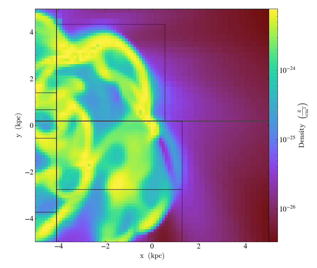
Overplot Grids

annotate_grids(self, alpha=0.7, min_pix=1, min_pix_ids=20, draw_ids=False, id_loc='lower left', periodic=True, min_level=None, max_level=None, cmap='B-W Linear_r', edgecolors=None, linewidth=1.0)

(This is a proxy for GridBoundaryCallback.)

Adds grid boundaries to a plot, optionally with alpha-blending via the alpha keyword. Cuttoff for display is at min_pix wide. draw_ids puts the grid id in the id_loc corner of the grid. (id_loc can be upper/lower left/right. draw_ids is not so great in projections…)

import yt

ds = yt.load("IsolatedGalaxy/galaxy0030/galaxy0030")
slc = yt.SlicePlot(ds, "z", ("gas", "density"), width=(10, "kpc"), center="max")
slc.annotate_grids()
slc.save()

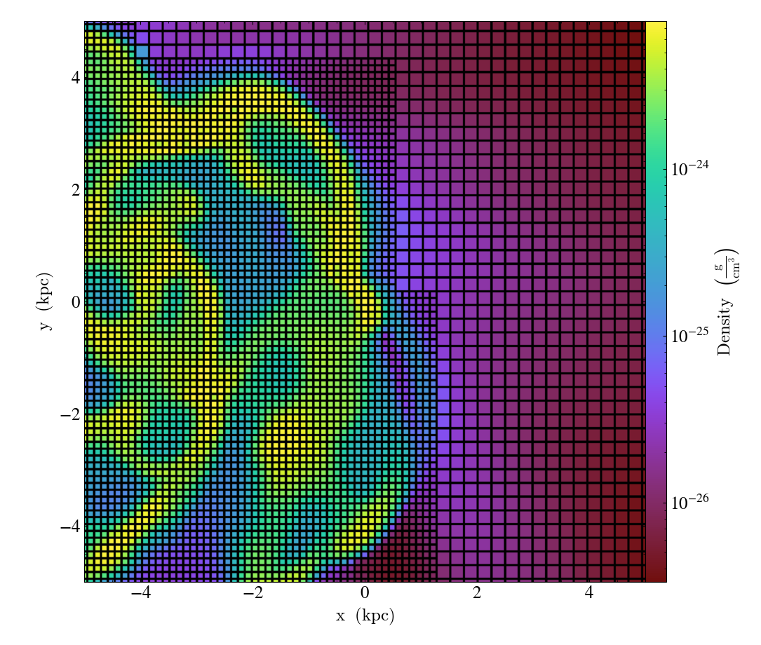
Overplot Cell Edges

annotate_cell_edges(line_width=0.002, alpha=1.0, color='black')

(This is a proxy for CellEdgesCallback.)

Annotate the edges of cells, where the line_width relative to size of the longest plot axis is specified. The alpha of the overlaid image and the color of the lines are also specifiable. Note that because the lines are drawn from both sides of a cell, the image sometimes has the effect of doubling the line width. Color here is a matplotlib color name or a 3-tuple of RGB float values.

import yt

ds = yt.load("IsolatedGalaxy/galaxy0030/galaxy0030")
slc = yt.SlicePlot(ds, "z", ("gas", "density"), width=(10, "kpc"), center="max")
slc.annotate_cell_edges()
slc.save()

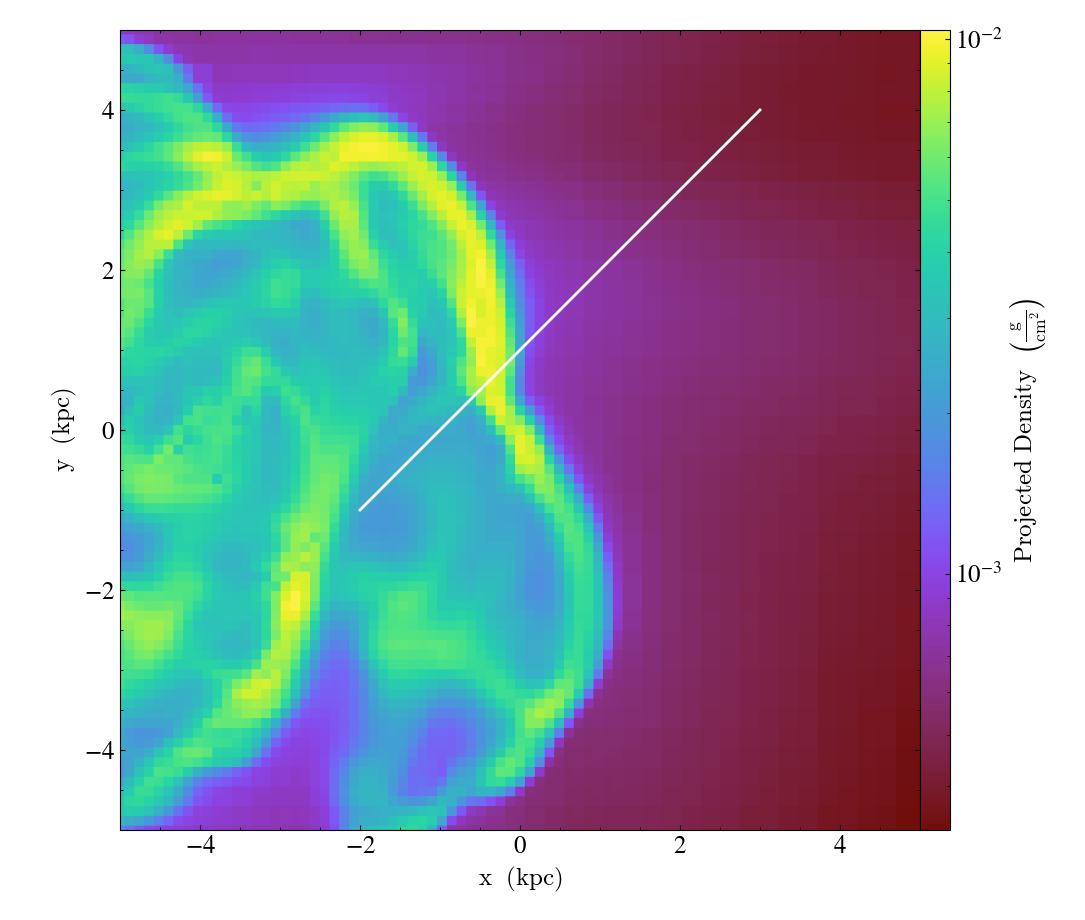
Overplot a Straight Line

annotate_line(self, p1, p2, *, coord_system='data', **kwargs)

(This is a proxy for LinePlotCallback.)

Overplot a line with endpoints at p1 and p2. p1 and p2 should be 2D or 3D coordinates consistent with the coordinate system denoted in the “coord_system” keyword.

import yt

ds = yt.load("IsolatedGalaxy/galaxy0030/galaxy0030")
p = yt.ProjectionPlot(ds, "z", ("gas", "density"), center="m", width=(10, "kpc"))
p.annotate_line((0.3, 0.4), (0.8, 0.9), coord_system="axis")
p.save()

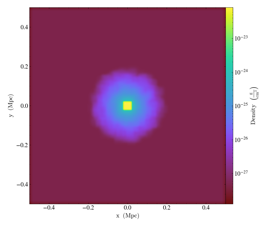
Overplot Magnetic Field Quivers

annotate_magnetic_field(self, factor=16, *, scale=None, scale_units=None, normalize=False, **kwargs)

(This is a proxy for MagFieldCallback.)

Adds a ‘quiver’ plot of magnetic field to the plot, skipping every factor datapoints in the discretization. scale is the data units per arrow length unit using scale_units. If normalize is True, the magnetic fields will be scaled by their local (in-plane) length, allowing morphological features to be more clearly seen for fields with substantial variation in field strength. Additional arguments can be passed to the plot_args dictionary, see matplotlib.axes.Axes.quiver for more info.

import yt

ds = yt.load(
    "MHDSloshing/virgo_low_res.0054.vtk",
    units_override={
        "time_unit": (1, "Myr"),
        "length_unit": (1, "Mpc"),
        "mass_unit": (1e17, "Msun"),
    },
)
p = yt.ProjectionPlot(ds, "z", ("gas", "density"), center="c", width=(300, "kpc"))
p.annotate_magnetic_field(headlength=3)
p.save()

Annotate a Point With a Marker

annotate_marker(self, pos, marker='x', *, coord_system='data', **kwargs)

(This is a proxy for MarkerAnnotateCallback.)

Overplot a marker on a position for highlighting specific features.

import yt

ds = yt.load("IsolatedGalaxy/galaxy0030/galaxy0030")
s = yt.SlicePlot(ds, "z", ("gas", "density"), center="c", width=(10, "kpc"))
s.annotate_marker((-2, -2), coord_system="plot", color="blue", s=500)
s.save()

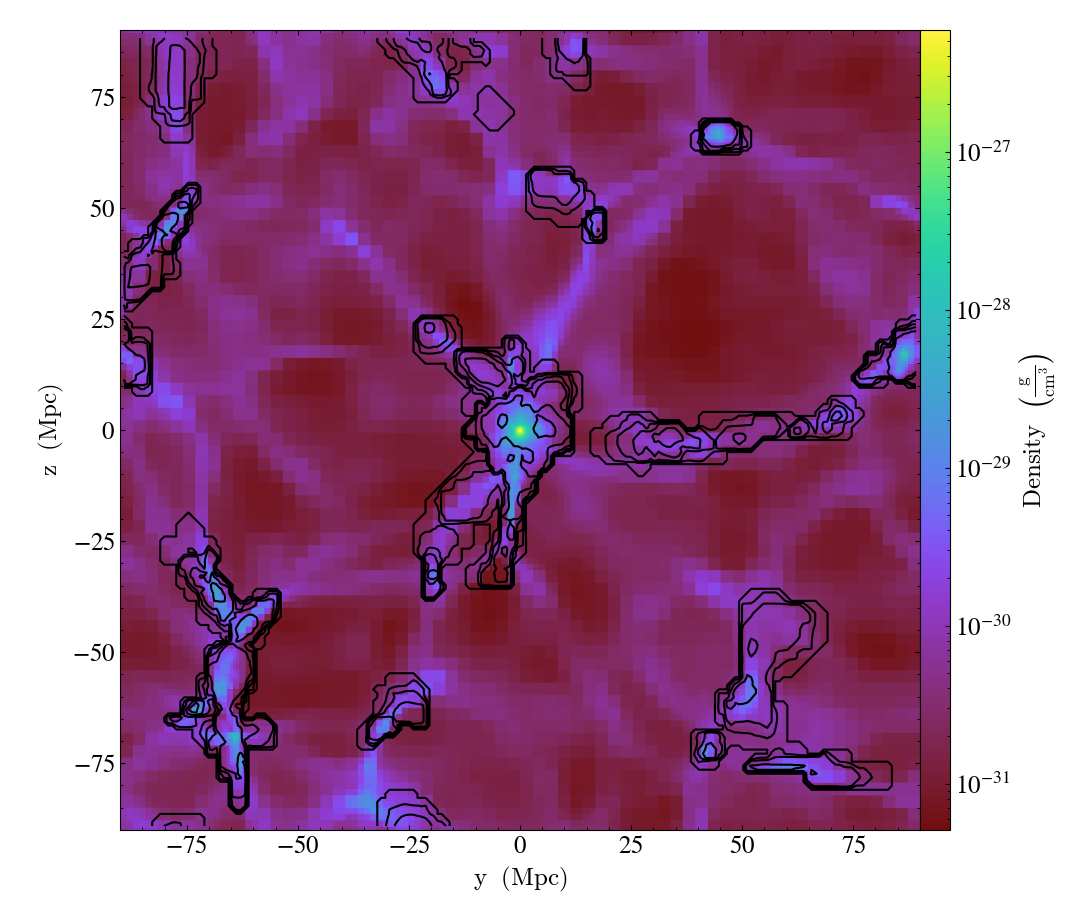
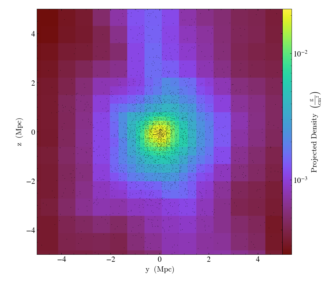
Overplotting Particle Positions

annotate_particles(self, width, p_size=1.0, col='k', marker='o', stride=1, ptype='all', alpha=1.0, data_source=None)

(This is a proxy for ParticleCallback.)

Adds particle positions, based on a thick slab along axis with a width along the line of sight. p_size controls the number of pixels per particle, and col governs the color. ptype will restrict plotted particles to only those that are of a given type. data_source will only plot particles contained within the data_source object.

WARNING: if data_source is a yt.data_objects.selection_data_containers.YTCutRegion then the width parameter is ignored.

import yt

ds = yt.load("Enzo_64/DD0043/data0043")
p = yt.ProjectionPlot(ds, "x", ("gas", "density"), center="m", width=(10, "Mpc"))
p.annotate_particles((10, "Mpc"))
p.save()

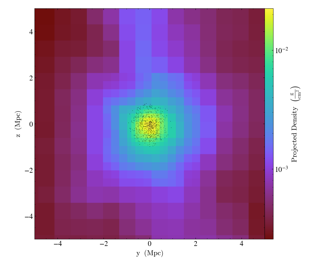
To plot only the central particles

import yt

ds = yt.load("Enzo_64/DD0043/data0043")
p = yt.ProjectionPlot(ds, "x", ("gas", "density"), center="m", width=(10, "Mpc"))
sp = ds.sphere(p.data_source.center, ds.quan(1, "Mpc"))
p.annotate_particles((10, "Mpc"), data_source=sp)
p.save()

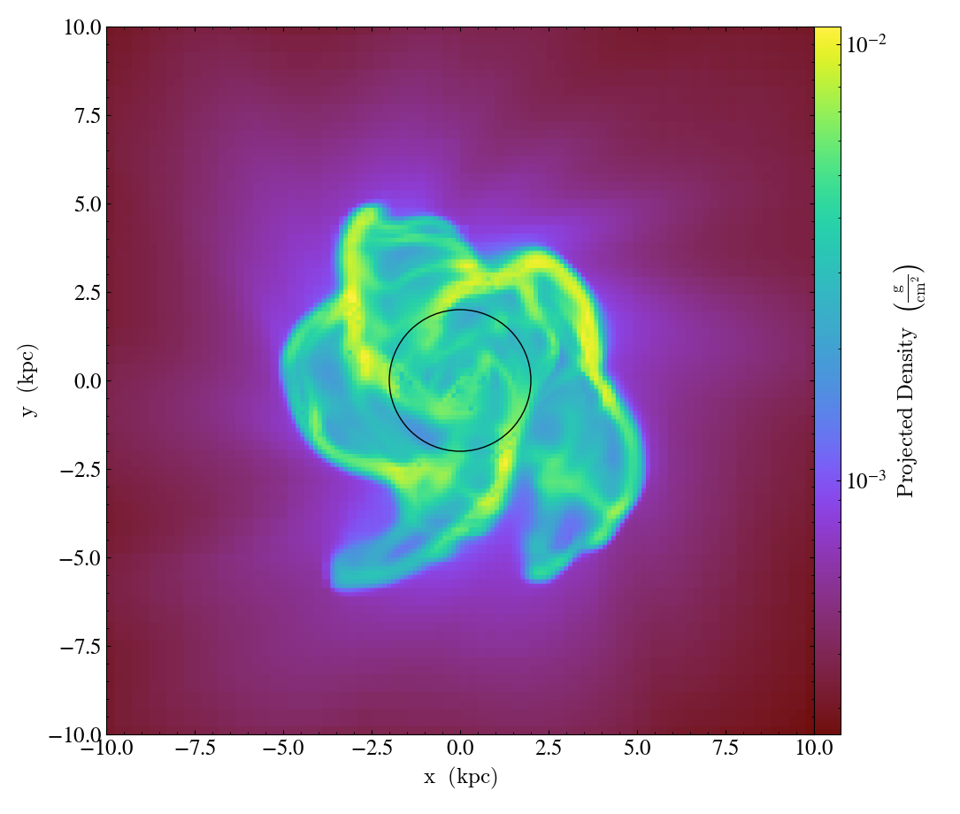
Overplot a Circle on a Plot

annotate_sphere(self, center, radius, circle_args=None, coord_system='data', text=None, text_args=None)

(This is a proxy for SphereCallback.)

Overplot a circle with designated center and radius with optional text.

import yt

ds = yt.load("IsolatedGalaxy/galaxy0030/galaxy0030")
p = yt.ProjectionPlot(ds, "z", ("gas", "density"), center="c", width=(20, "kpc"))
p.annotate_sphere([0.5, 0.5, 0.5], radius=(2, "kpc"), circle_args={"color": "black"})
p.save()

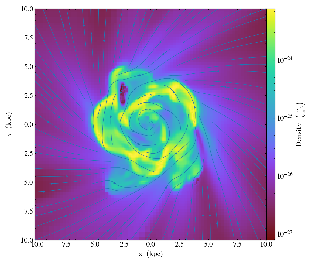
Overplot Streamlines

annotate_streamlines(self, field_x, field_y, *, linewidth=1.0, linewidth_upscaling=1.0, color=None, color_threshold=float('-inf'), factor=16, **kwargs)

(This is a proxy for StreamlineCallback.)

Add streamlines to any plot, using the field_x and field_y from the associated data, using nx and ny starting points that are bounded by xstart and ystart. To begin streamlines from the left edge of the plot, set start_at_xedge to True; for the bottom edge, use start_at_yedge. A line with the qmean vector magnitude will cover 1.0/factor of the image.

Additional keyword arguments are passed down to matplotlib.axes.Axes.streamplot

import yt

ds = yt.load("IsolatedGalaxy/galaxy0030/galaxy0030")
s = yt.SlicePlot(ds, "z", ("gas", "density"), center="c", width=(20, "kpc"))
s.annotate_streamlines(("gas", "velocity_x"), ("gas", "velocity_y"))
s.save()

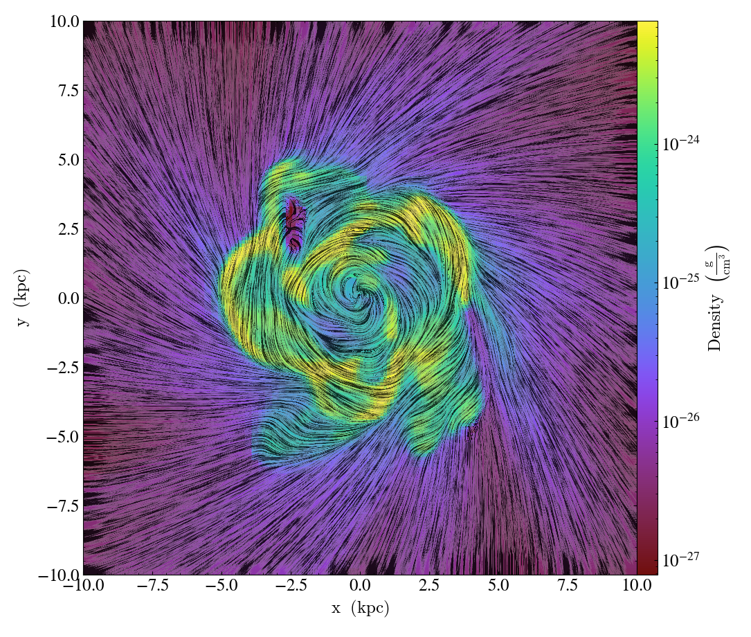
Overplot Line Integral Convolution

annotate_line_integral_convolution(self, field_x, field_y, texture=None, kernellen=50., lim=(0.5, 0.6), cmap='binary', alpha=0.8, const_alpha=False)

(This is a proxy for LineIntegralConvolutionCallback.)

Add line integral convolution to any plot, using the field_x and field_y from the associated data. A white noise background will be used for texture as default. Adjust the bounds of lim in the range of [0, 1] which applies upper and lower bounds to the values of line integral convolution and enhance the visibility of plots. When const_alpha=False, alpha will be weighted spatially by the values of line integral convolution; otherwise a constant value of the given alpha is used.

import yt

ds = yt.load("IsolatedGalaxy/galaxy0030/galaxy0030")
s = yt.SlicePlot(ds, "z", ("gas", "density"), center="c", width=(20, "kpc"))
s.annotate_line_integral_convolution(("gas", "velocity_x"), ("gas", "velocity_y"), lim=(0.5, 0.65))
s.save()

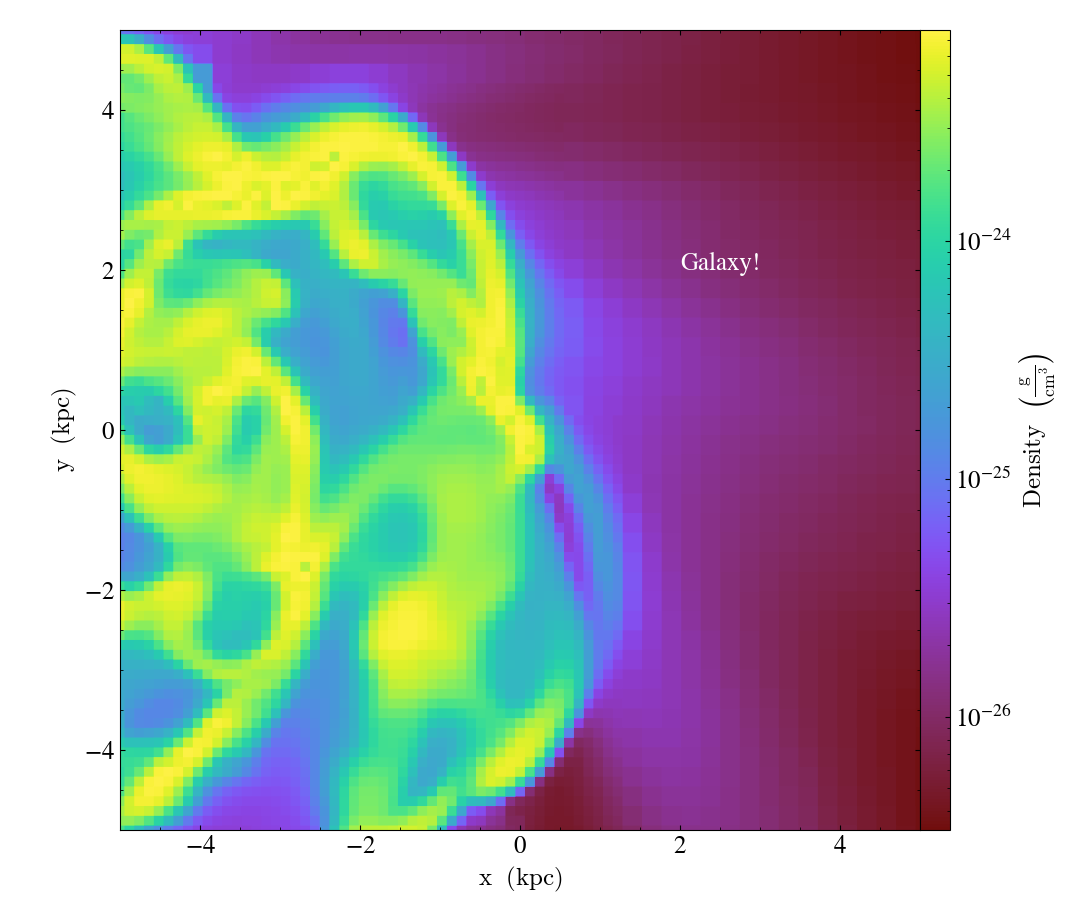
Overplot Text

annotate_text(self, pos, text, coord_system='data', text_args=None, inset_box_args=None)

(This is a proxy for TextLabelCallback.)

Overplot text on the plot at a specified position. If you desire an inset box around your text, set one with the inset_box_args dictionary keyword.

import yt

ds = yt.load("IsolatedGalaxy/galaxy0030/galaxy0030")
s = yt.SlicePlot(ds, "z", ("gas", "density"), center="max", width=(10, "kpc"))
s.annotate_text((2, 2), "Galaxy!", coord_system="plot")
s.save()

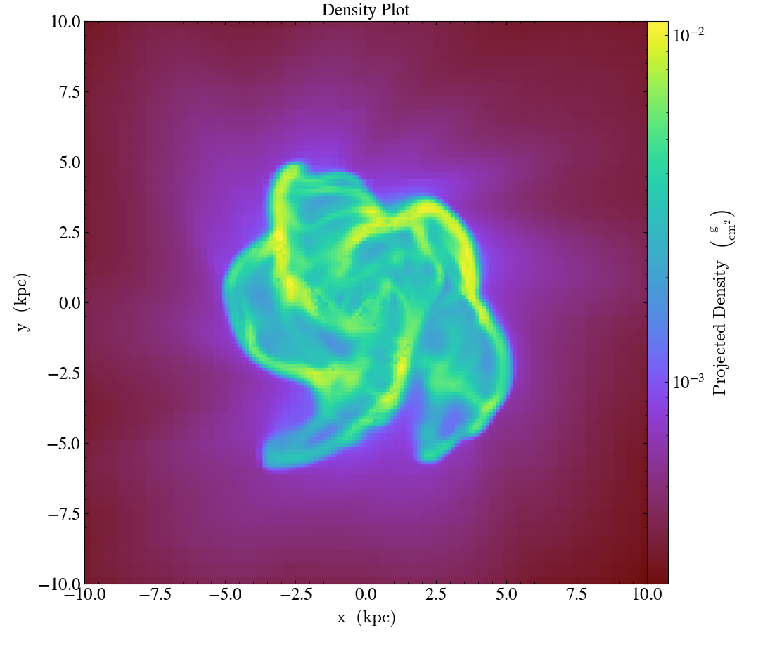
Add a Title

annotate_title(self, title='Plot')

(This is a proxy for TitleCallback.)

Accepts a title and adds it to the plot.

import yt

ds = yt.load("IsolatedGalaxy/galaxy0030/galaxy0030")
p = yt.ProjectionPlot(ds, "z", ("gas", "density"), center="c", width=(20, "kpc"))
p.annotate_title("Density Plot")
p.save()

Overplot Quivers for the Velocity Field

annotate_velocity(self, factor=16, *, scale=None, scale_units=None, normalize=False, **kwargs)

(This is a proxy for VelocityCallback.)

Adds a ‘quiver’ plot of velocity to the plot, skipping every factor datapoints in the discretization. scale is the data units per arrow length unit using scale_units. If normalize is True, the velocity fields will be scaled by their local (in-plane) length, allowing morphological features to be more clearly seen for fields with substantial variation in field strength. Additional arguments can be passed to the plot_args dictionary, see matplotlib.axes.Axes.quiver for more info.

import yt

ds = yt.load("IsolatedGalaxy/galaxy0030/galaxy0030")
p = yt.SlicePlot(ds, "z", ("gas", "density"), center="m", width=(10, "kpc"))
p.annotate_velocity(headwidth=4)
p.save()

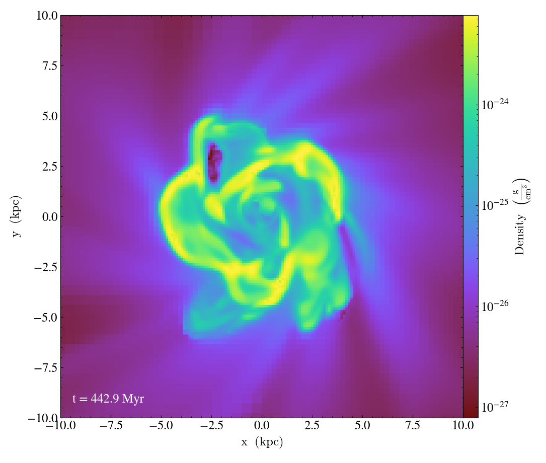
Add the Current Time and/or Redshift

annotate_timestamp(x_pos=None, y_pos=None, corner='lower_left', time=True, redshift=False, time_format='t = {time:.1f} {units}', time_unit=None, time_offset=None, redshift_format='z = {redshift:.2f}', draw_inset_box=False, coord_system='axis', text_args=None, inset_box_args=None)

(This is a proxy for TimestampCallback.)

Annotates the timestamp and/or redshift of the data output at a specified location in the image (either in a present corner, or by specifying (x,y) image coordinates with the x_pos, y_pos arguments. If no time_units are specified, it will automatically choose appropriate units. It allows for custom formatting of the time and redshift information, the specification of an inset box around the text, and changing the value of the timestamp via a constant offset.

import yt

ds = yt.load("IsolatedGalaxy/galaxy0030/galaxy0030")
p = yt.SlicePlot(ds, "z", ("gas", "density"), center="c", width=(20, "kpc"))
p.annotate_timestamp()
p.save()

Add a Physical Scale Bar

annotate_scale(corner='lower_right', coeff=None, unit=None, pos=None, scale_text_format='{scale} {units}', max_frac=0.16, min_frac=0.015, coord_system='axis', text_args=None, size_bar_args=None, draw_inset_box=False, inset_box_args=None)

(This is a proxy for ScaleCallback.)

Annotates the scale of the plot at a specified location in the image (either in a preset corner, or by specifying (x,y) image coordinates with the pos argument. Coeff and units (e.g. 1 Mpc or 100 kpc) refer to the distance scale you desire to show on the plot. If no coeff and units are specified, an appropriate pair will be determined such that your scale bar is never smaller than min_frac or greater than max_frac of your plottable axis length. Additional customization of the scale bar is possible by adjusting the text_args and size_bar_args dictionaries. The text_args dictionary accepts matplotlib’s font_properties arguments to override the default font_properties for the current plot. The size_bar_args dictionary accepts keyword arguments for the AnchoredSizeBar class in matplotlib’s axes_grid toolkit. Finally, the format of the scale bar text can be adjusted using the scale_text_format keyword argument.

import yt

ds = yt.load("IsolatedGalaxy/galaxy0030/galaxy0030")
p = yt.SlicePlot(ds, "z", ("gas", "density"), center="c", width=(20, "kpc"))
p.annotate_scale()
p.save()

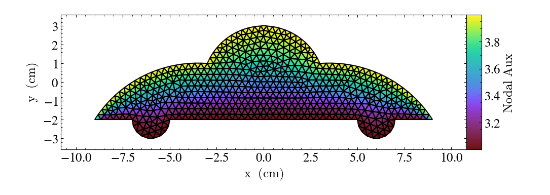
Annotate Triangle Facets Callback

annotate_triangle_facets(triangle_vertices, **kwargs)

(This is a proxy for TriangleFacetsCallback.)

This add a line collection of a SlicePlot’s plane-intersection with the triangles to the plot. This callback is ideal for a dataset representing a geometric model of triangular facets.

import os

import h5py

import yt

# Load data file
ds = yt.load("MoabTest/fng_usrbin22.h5m")

# Create the desired slice plot
s = yt.SlicePlot(ds, "z", ("moab", "TALLY_TAG"))

# get triangle vertices from file (in this case hdf5)

# setup file path for yt test directory
filename = os.path.join(
    yt.config.ytcfg.get("yt", "test_data_dir"), "MoabTest/mcnp_n_impr_fluka.h5m"
)
f = h5py.File(filename, mode="r")
coords = f["/tstt/nodes/coordinates"][:]
conn = f["/tstt/elements/Tri3/connectivity"][:]
points = coords[conn - 1]

# Annotate slice-triangle intersection contours to the plot
s.annotate_triangle_facets(points, colors="black")
s.save()

Annotate Mesh Lines Callback

annotate_mesh_lines(**kwargs)

(This is a proxy for MeshLinesCallback.)

This draws the mesh line boundaries over a plot using a Matplotlib line collection. This callback is only useful for unstructured or semi-structured mesh datasets.

import yt

ds = yt.load("MOOSE_sample_data/out.e")
sl = yt.SlicePlot(ds, "z", ("connect1", "nodal_aux"))
sl.annotate_mesh_lines(color="black")
sl.save()

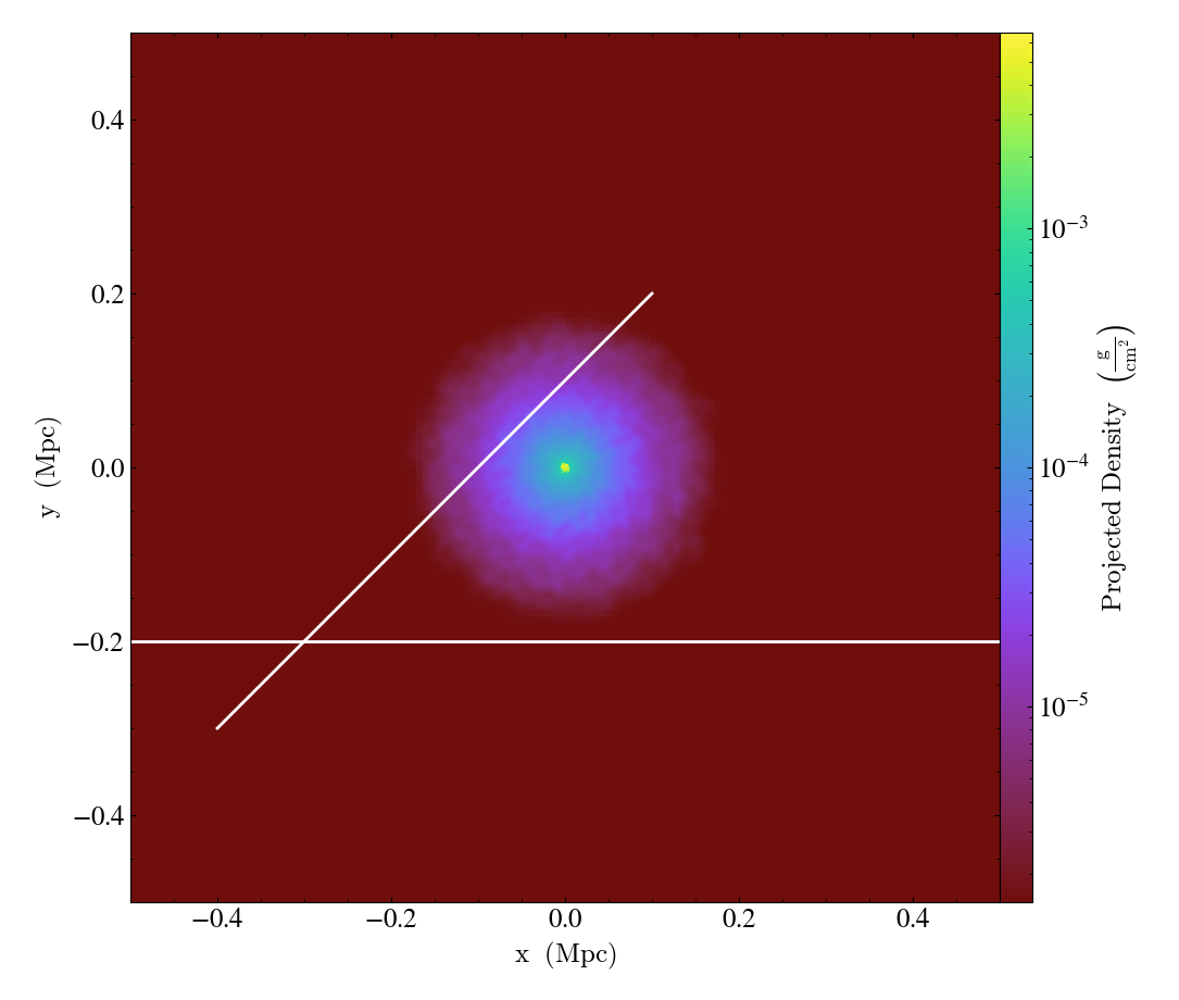
Overplot the Path of a Ray

annotate_ray(ray, *, arrow=False, **kwargs)

(This is a proxy for RayCallback.)

Adds a line representing the projected path of a ray across the plot. The ray can be either a YTOrthoRay, YTRay, or a Trident LightRay object. annotate_ray() will properly account for periodic rays across the volume.

import yt

ds = yt.load("IsolatedGalaxy/galaxy0030/galaxy0030")
oray = ds.ortho_ray(0, (0.3, 0.4))
ray = ds.ray((0.1, 0.2, 0.3), (0.6, 0.7, 0.8))
p = yt.ProjectionPlot(ds, "z", ("gas", "density"))
p.annotate_ray(oray)
p.annotate_ray(ray)
p.save()

Applying filters on the final image

It is also possible to operate on the plotted image directly by using one of the fixed resolution buffer filter as described in Fixed Resolution Buffer Filters. Note that it is necessary to call the plot object’s refresh method to apply filters.

import yt

ds = yt.load('IsolatedGalaxy/galaxy0030/galaxy0030')
p = yt.SlicePlot(ds, 'z', 'density')
p.frb.apply_gauss_beam(sigma=30)
p.refresh()
p.save()

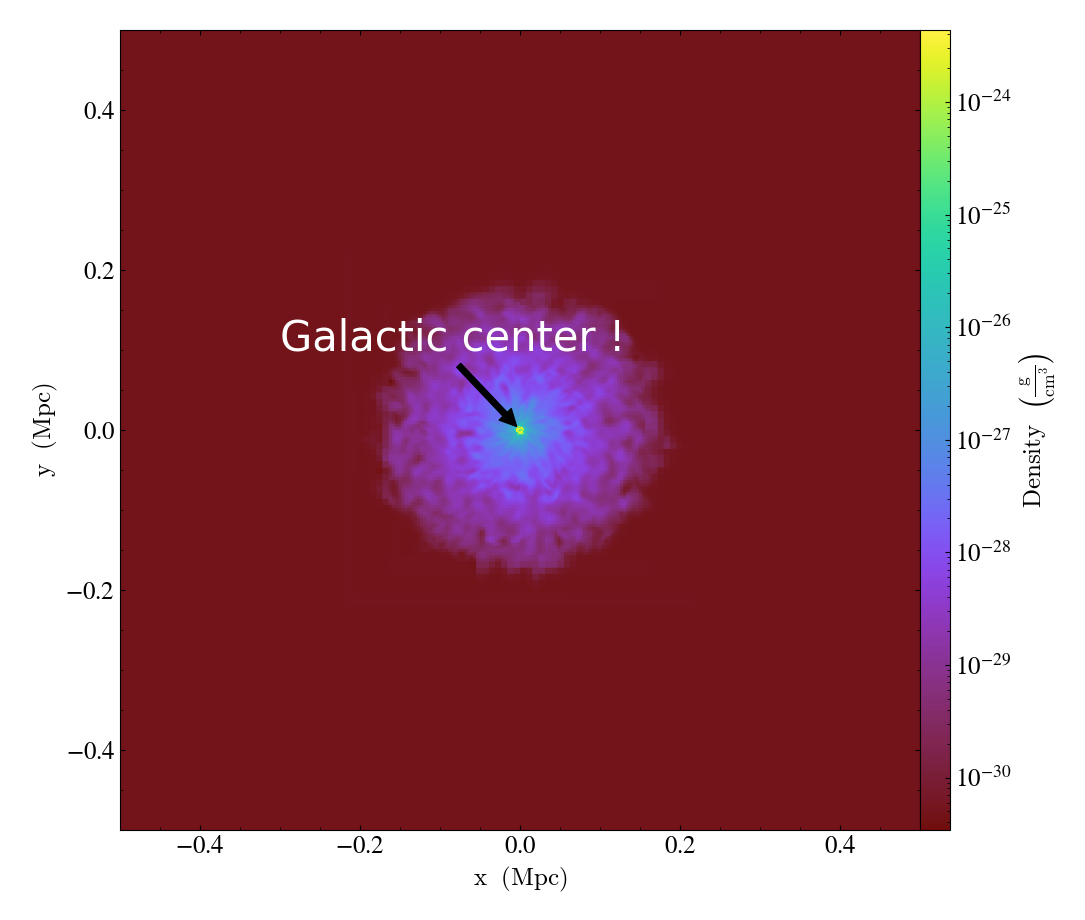
Extending annotations methods

New annotate_ methods can be added to plot objects at runtime (i.e., without modifying yt’s source code) by subclassing the base PlotCallback class. This is the recommended way to add custom and unique annotations to yt plots, as it can be done through local plugins, individual scripts, or even external packages.

Here’s a minimal example:

import yt
from yt.visualization.api import PlotCallback


class TextToPositionCallback(PlotCallback):
   # bind a new `annotate_text_to_position` plot method
   _type_name = "text_to_position"

   def __init__(self, text, x, y):
      # this method can have arbitrary arguments
      # and should store them without alteration,
      # but not run expensive computations
      self.text = text
      self.position = (x, y)

   def __call__(self, plot):
      # this method's signature is required
      # this is where we perform potentially expensive operations

      # the plot argument exposes matplotlib objects:
      # - plot._axes is a matplotlib.axes.Axes object
      # - plot._figure is a matplotlib.figure.Figure object
      plot._axes.annotate(
            self.text,
            xy=self.position,
            xycoords="data",
            xytext=(0.2, 0.6),
            textcoords="axes fraction",
            color="white",
            fontsize=30,
            arrowprops=dict(facecolor="black", shrink=0.05),
      )

ds = yt.load("IsolatedGalaxy/galaxy0030/galaxy0030")
p = yt.SlicePlot(ds, "z", "density")
p.annotate_text_to_position("Galactic center !", x=0, y=0)
p.save()