Constructing Data Objects
These recipes demonstrate a few uncommon methods of constructing data objects from a simulation.
Creating Particle Filters
Create particle filters based on the age of star particles in an isolated disk galaxy simulation. Determine the total mass of each stellar age bin in the simulation. Generate projections for each of the stellar age bins.
import numpy as np

import yt
from yt.data_objects.particle_filters import add_particle_filter


# Define filter functions for our particle filters based on stellar age.
# In this dataset particles in the initial conditions are given creation
# times arbitrarily far into the future, so stars with negative ages belong
# in the old stars filter.
def stars_10Myr(pfilter, data):
    age = data.ds.current_time - data["Stars", "creation_time"]
    filter = np.logical_and(age >= 0, age.in_units("Myr") < 10)
    return filter


def stars_100Myr(pfilter, data):
    age = (data.ds.current_time - data["Stars", "creation_time"]).in_units("Myr")
    filter = np.logical_and(age >= 10, age < 100)
    return filter


def stars_old(pfilter, data):
    age = data.ds.current_time - data["Stars", "creation_time"]
    filter = np.logical_or(age < 0, age.in_units("Myr") >= 100)
    return filter


# Create the particle filters
add_particle_filter(
    "stars_young",
    function=stars_10Myr,
    filtered_type="Stars",
    requires=["creation_time"],
)
add_particle_filter(
    "stars_medium",
    function=stars_100Myr,
    filtered_type="Stars",
    requires=["creation_time"],
)
add_particle_filter(
    "stars_old", function=stars_old, filtered_type="Stars", requires=["creation_time"]
)

# Load a dataset and apply the particle filters
filename = "TipsyGalaxy/galaxy.00300"
ds = yt.load(filename)
ds.add_particle_filter("stars_young")
ds.add_particle_filter("stars_medium")
ds.add_particle_filter("stars_old")

# What are the total masses of different ages of star in the whole simulation
# volume?
ad = ds.all_data()
mass_young = ad["stars_young", "particle_mass"].in_units("Msun").sum()
mass_medium = ad["stars_medium", "particle_mass"].in_units("Msun").sum()
mass_old = ad["stars_old", "particle_mass"].in_units("Msun").sum()
print(f"Mass of young stars = {mass_young:g}")
print(f"Mass of medium stars = {mass_medium:g}")
print(f"Mass of old stars = {mass_old:g}")

# Generate 4 projections: gas density, young stars, medium stars, old stars
fields = [
    ("stars_young", "particle_mass"),
    ("stars_medium", "particle_mass"),
    ("stars_old", "particle_mass"),
]

prj1 = yt.ProjectionPlot(ds, "z", ("gas", "density"), center="max", width=(100, "kpc"))
prj1.save()
prj2 = yt.ParticleProjectionPlot(ds, "z", fields, center="max", width=(100, "kpc"))
prj2.save()

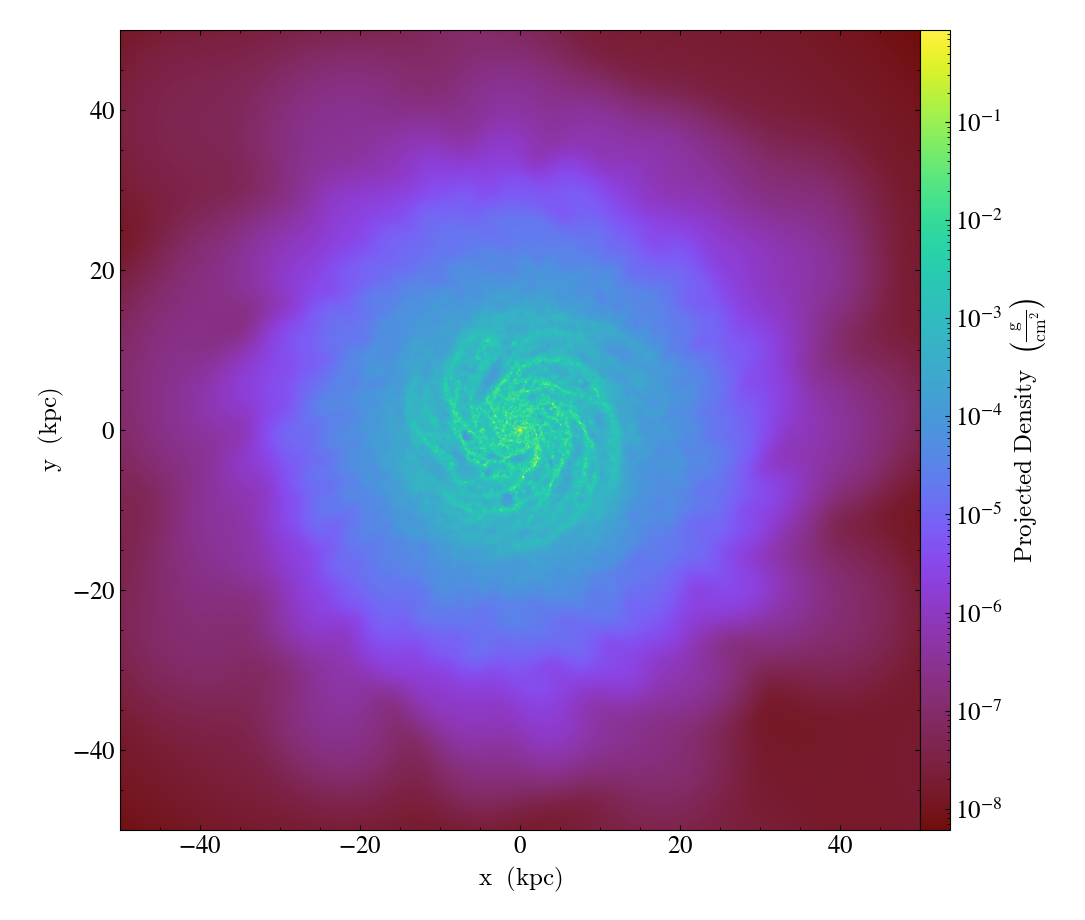
Identifying Clumps
This is a recipe to show how to find topologically connected sets of cells inside a dataset. It returns these clumps and they can be inspected or visualized as would any other data object. More detail on this method can be found in Smith et al. 2009.
import numpy as np
import yt
from yt.data_objects.level_sets.api import Clump, find_clumps
ds = yt.load("IsolatedGalaxy/galaxy0030/galaxy0030")
data_source = ds.disk([0.5, 0.5, 0.5], [0.0, 0.0, 1.0], (8, "kpc"), (1, "kpc"))
# the field to be used for contouring
field = ("gas", "density")
# This is the multiplicative interval between contours.
step = 2.0
# Now we set some sane min/max values between which we want to find contours.
# This is how we tell the clump finder what to look for -- it won't look for
# contours connected below or above these threshold values.
c_min = 10 ** np.floor(np.log10(data_source[field]).min())
c_max = 10 ** np.floor(np.log10(data_source[field]).max() + 1)
# Now find get our 'base' clump -- this one just covers the whole domain.
master_clump = Clump(data_source, field)
# Add a "validator" to weed out clumps with less than 20 cells.
# As many validators can be added as you want.
master_clump.add_validator("min_cells", 20)
# Calculate center of mass for all clumps.
master_clump.add_info_item("center_of_mass")
# Begin clump finding.
find_clumps(master_clump, c_min, c_max, step)
# Save the clump tree as a reloadable dataset
fn = master_clump.save_as_dataset(fields=[("gas", "density"), ("all", "particle_mass")])
# We can traverse the clump hierarchy to get a list of all of the 'leaf' clumps
leaf_clumps = master_clump.leaves
# Get total cell and particle masses for each leaf clump
leaf_masses = [leaf.quantities.total_mass() for leaf in leaf_clumps]
# If you'd like to visualize these clumps, a list of clumps can be supplied to
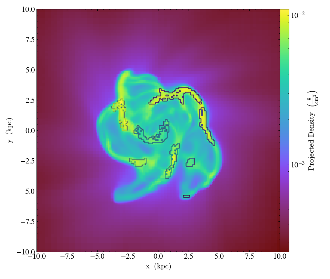
# the "clumps" callback on a plot. First, we create a projection plot:
prj = yt.ProjectionPlot(ds, 2, field, center="c", width=(20, "kpc"))
# Next we annotate the plot with contours on the borders of the clumps
prj.annotate_clumps(leaf_clumps)
# Save the plot to disk.
prj.save("clumps")
# Reload the clump dataset.
cds = yt.load(fn)
# Clump annotation can also be done with the reloaded clump dataset.
# Remove the original clump annotation
prj.clear_annotations()
# Get the leaves and add the callback.
leaf_clumps_reloaded = cds.leaves
prj.annotate_clumps(leaf_clumps_reloaded)
prj.save("clumps_reloaded")
# Query fields for clumps in the tree.
print(cds.tree["clump", "center_of_mass"])
print(cds.tree.children[0]["grid", "density"])
print(cds.tree.children[1]["all", "particle_mass"])
# Get all of the leaf clumps.
print(cds.leaves)
print(cds.leaves[0]["clump", "cell_mass"])

Extracting Fixed Resolution Data
This is a recipe to show how to open a dataset and extract it to a file at a fixed resolution with no interpolation or smoothing. Additionally, this recipe shows how to insert a dataset into an external HDF5 file using h5py.
(extract_fixed_resolution_data.py)
# For this example we will use h5py to write to our output file.
import h5py

import yt

ds = yt.load("IsolatedGalaxy/galaxy0030/galaxy0030")

level = 2
dims = ds.domain_dimensions * ds.refine_by**level

# We construct an object that describes the data region and structure we want
# In this case, we want all data up to the maximum "level" of refinement
# across the entire simulation volume.  Higher levels than this will not
# contribute to our covering grid.
cube = ds.covering_grid(
    level,
    left_edge=[0.0, 0.0, 0.0],
    dims=dims,
    # And any fields to preload (this is optional!)
    fields=[("gas", "density")],
)

# Now we open our output file using h5py
# Note that we open with 'w' (write), which will overwrite existing files!
f = h5py.File("my_data.h5", mode="w")

# We create a dataset at the root, calling it "density"
f.create_dataset("/density", data=cube["gas", "density"])

# We close our file
f.close()

# If we want to then access this datacube in the h5 file, we can now...
f = h5py.File("my_data.h5", mode="r")
print(f["density"][()])