How Particles are Indexed

With yt-4.0, the method by which particles are indexed changed considerably. Whereas in previous versions, particles were indexed based on their position in an octree (the structure of which was determined by particle number density), in yt-4.0 this system was overhauled to utilize a bitmap index based on a space-filling curve, using a enhanced word-aligned hybrid boolean array as their backend.

Note

You may see scattered references to “the demeshening” (including in the filename for this document!). This was a humorous name used in the yt development process to refer to removing a global (octree) mesh for particle codes.

By avoiding the use of octrees as a base mesh, yt is able to create much more accurate SPH visualizations. We have a gallery demonstrating this but even in this side-by-side comparison the differences can be seen quite easily, with the left image being from the old, octree-based approach and the right image the new, meshless approach.

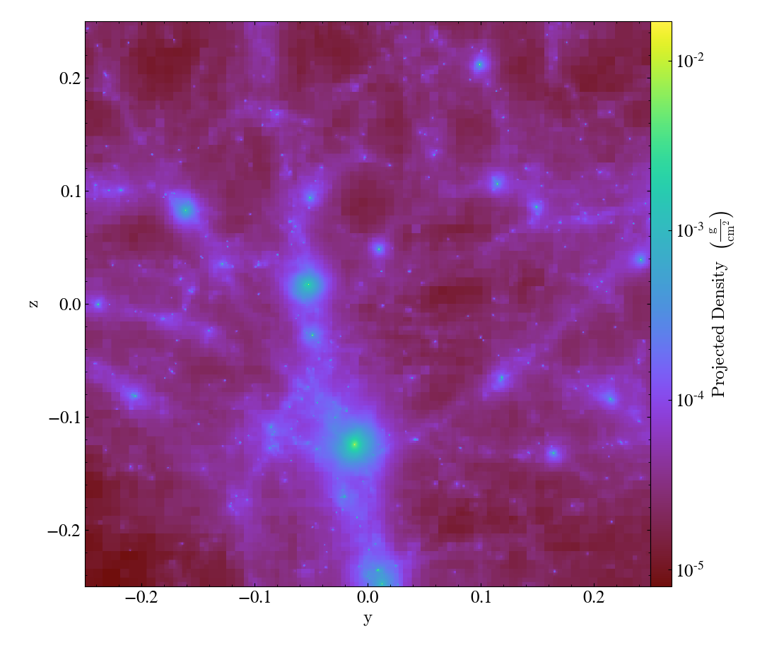
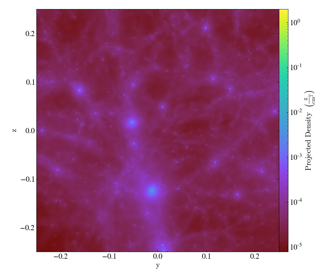
Effectively, what “the demeshening” does is allow yt to treat the particles as discrete objects (or with an area of influence) and use their positions in a multi-level index to optimize and minimize the disk operations necessary to load only those particles it needs.

Note

The theory and implementation of yt’s bitmap indexing system is described in some detail in the yt 4.0 paper in the section entitled Indexing Discrete-Point Datasets.

In brief, however, what this relies on is two numbers, index_order1 and index_order2. These control the “coarse” and “refined” sets of indices, and they are supplied to any particle dataset load() in the form of a tuple as the argument index_order. By default these are set to 5 and 7, respectively, but it is entirely likely that a different set of values will work better for your purposes.

For example, if you were to use the sample Gadget-3 dataset, you could override the default values and use values of 5 and 5 by specifying this argument to the load_sample function; this works with load as well.

ds = yt.load_sample("Gadget3-snap-format2", index_order=(5, 5))

So this is how you change the index order, but it doesn’t explain precisely what this “index order” actually is.

Indexing and Why yt Does it

yt is based on the idea that data should be selected and read only when it is needed. So for instance, if you only want particles or grid cells from a small region in the center of your dataset, yt wants to avoid any reading of the data outside of that region. Now, in practice, this isn’t entirely possible – particularly with particles, you can’t actually tell when something is inside or outside of a region until you read it, because the particle locations are stored in the dataset.

One way to avoid this is to have an index of the data, so that yt can know that some of the data that is located here in space is located there in the file or files on disk. So if you’re able to say, I only care about data in “region A”, you can look for those files that contain data within “region A,” read those, and discard the parts of them that are not within “region A.”

The finer grained the index, the longer it takes to build that index – and the larger than index is, and the longer it takes to query. The cost of having too coarse an index, on the other hand, is that the IO conducted to read a given region is likely to be too much, and more particles will be discarded after being read, before being “selected” by the data selector (sphere, region, etc).

An important note about all of this is that the index system is not meant to replace the positions stored on disk, but instead to speed up queries of those positions – the index is meant to be lossy in representation, and only provides means of generating IO information. Additionally, the atomic unit that yt considers when conducting IO or selection queries is called a “chunk” internally. For situations where the individual files are very, very large, yt will “sub-chunk” these into smaller bits, which are by-default set to $64^3$ particles. Whenever indexing is done, it is done at this granular level, with offsets to individual particle collections stored. For instance, if you had a (single) file with $1024^3$ particles in it, yt would instead regard this as a series of $64^3$ particle files, and index each one individually.

Index Order

The bitmap index system is based on a two-level scheme for assigning positions in three-dimensional space to integer values. What this means is that each particle is assigned a “coarse” index, which is global to the full domain of the collection of particles, and if necessary an additional “refined” index is assigned to the particle, within that coarse index.

The index “order” values refer to the number of entries on a side that each index system is allowed. For instance, if we allow the particles to be subdivided into 8 “bins” in each direction, this would correspond to an index order of 3 (as $2^3 = 8$); correspondingly, an index order of 5 would be 32 bins in each direction, and an index order of 7 would be 128 bins in each direction. Each particle is then assigned a set of i, j, k values for the bin value in each dimension, and these i, j, k values are combined into a single (64-bit) integer according to a space-filling curve.

The process by which this is done by yt is as follows:

1. For each “chunk” of data – which may be a file, or a subset of a file in which particles are contained – assign each particle to an integer value according to the space-filling curve and the coarse index order. Set the “bit” in an array of boolean values that each of these integers correspond to. Note that this is almost certainly reductive – there will be fewer bits set than there are particles, which is by design.

2. Once all chunks or files have been assigned an array of bits that correspond to the places where, according to the coarse indexing scheme, they have particles, identify all those “bits” that have been set by more than one chunk. All of these bits correspond to locations where more than one file contains particles – so if you want to select something from this region, you’d need to read more than one file.

3. For each “collision” location, apply a second-order index, to identify which sub-regions are touched by more than one file.

At the end of this process, each file will be associated with a single “coarse” index (which covers the entire domain of the data), as well as a set of “collision” locations, and in each “collision” location a set of bitarrays that correspond to that subregion.

When reading data, yt will identify which “coarse” index regions are necessary to read. If any of those coarse index regions are covered by more than one file, it will examine the “refined” index for those regions and see if it is able to subset more efficiently. Because all of these operations can be done with logical operations, this considerably reduces the amount of data that needs to be read from disk before expensive selection operations are conducted.

For those situations that involve particles with regions of influence – such as smoothed particle hydrodynamics, where particles have associated smoothing lengths – these are taken into account when conducting the indexing system.

Efficiency of Index Orders

What this can lead to, however, is situations where (particularly at the edges of regions populated by SPH particles) the indexing system identifies collisions, but the relatively small number of particles and correspondingly large “smoothing lengths” result in a large number of “refined” index values that need to be set.

Counterintuitively, this actually means that occasionally the “refined” indexing process can take an inordinately long amount of time for small datasets, rather than large datasets.

In these situations, it is typically sufficient to set the “refined” index order to be much lower than its default value. For instance, setting the index_order to (5, 3) means that the full domain will be subdivided into 32 bins in each dimension, and any “collision” zones will be further subdivided into 8 bins in each dimension (corresponding to an effective 256 bins across the full domain).

If you are experiencing very long index times, this may be a productive parameter to modify. For instance, if you are seeing very rapid “coarse” indexing followed by very, very slow “refined” indexing, this likely plays a part; often this will be most obvious in small-ish (i.e., $256^3$ or smaller) datasets.

Index Caching

The index values are cached between instantiation, in a sidecar file named with the name of the dataset file and the suffix .indexII_JJ.ewah, where II and JJ are index_order1 and index_order2. So for instance, if index_order is set to (5, 7), and you are loading a dataset file named “snapshot_200.hdf5”, after indexing, you will have an index sidecar file named snapshot_200.hdf5.index5_7.ewah. On subsequent loads, this index file will be reused, rather than re-generated.

By default these sidecars are stored next to the dataset itself, in the same directory. However, the filename scheme (and thus location) can be changed by supplying an alternate filename to the load command with the argument index_filename. For instance, if you are accessing data in a read-only location, you can specify that the index will be cached in a location that is write-accessible to you.

These files contain the compressed bitmap index values, along with some metadata that describes the version of the indexing system they use and so forth. If the version of the index that yt uses has changed, they will be regenerated; in general this will not vary very often (and should be much less frequent than, for instance, yt releases) and yt will provide a message to let you know it is doing it.

The file size of these cached index files can be difficult to estimate; because it is based on a compressed bitmap arrays, it will depend on the spatial organization of the particles it is indexing, and how co-located they are according to the space filling curve. For very small datasets it will be small, but we do not expect these index files to grow beyond a few hundred megabytes even in the extreme case of large datasets that have little to no coherence in their clustering.