3D Surfaces and Sketchfab

Surface Objects and Extracting Isocontour Information

yt contains an implementation of the Marching Cubes algorithm, which can operate on 3D data objects. This provides two things. The first is to identify isocontours and return either the geometry of those isocontours or to return another field value sampled along that isocontour. The second piece of functionality is to calculate the flux of a field over an isocontour.

Note that these isocontours are not guaranteed to be topologically connected. In fact, inside a given data object, the marching cubes algorithm will return all isocontours, not just a single connected one. This means if you encompass two clumps of a given density in your data object and extract an isocontour at that density, it will include both of the clumps.

This means that with adaptive mesh refinement data, you will see cracks across refinement boundaries unless a “crack-fixing” step is applied to match up these boundaries. yt does not perform such an operation, and so there will be seams visible in 3D views of your isosurfaces.

Surfaces can be exported in OBJ format, values can be samples at the center of each face of the surface, and flux of a given field could be calculated over the surface. This means you can, for instance, extract an isocontour in density and calculate the mass flux over that isocontour. It also means you can export a surface from yt and view it in something like Blender, MeshLab, or even on your Android or iOS device in MeshPad.

To extract geometry or sample a field, call extract_isocontours(). To calculate a flux, call calculate_isocontour_flux(). both of these operations will run in parallel. For more information on enabling parallelism in yt, see Parallel Computation With yt.

Alternatively, you can make an object called YTSurface that makes this process much easier. You can create one of these objects by specifying a source data object and a field over which to identify a surface at a given value. For example:

import yt

ds = yt.load("IsolatedGalaxy/galaxy0030/galaxy0030")
sphere = ds.sphere("max", (1.0, "Mpc"))
surface = ds.surface(sphere, ("gas", "density"), 1e-27)

This object, surface, can be queried for values on the surface. For instance:

print(surface["gas", "temperature"].min(), surface["gas", "temperature"].max())

will return the values 11850.7476943 and 13641.0663899. These values are interpolated to the face centers of every triangle that constitutes a portion of the surface. Note that reading a new field requires re-calculating the entire surface, so it’s not the fastest operation. You can get the vertices of the triangle by looking at the property .vertices.

Exporting to a File

If you want to export this to a PLY file you can call the routine export_ply, which will write to a file and optionally sample a field at every face or vertex, outputting a color value to the file as well. This file can then be viewed in MeshLab, Blender or on the website Sketchfab.com. But if you want to view it on Sketchfab, there’s an even easier way!

Exporting to Sketchfab

Sketchfab is a website that uses WebGL, a relatively new technology for displaying 3D graphics in any browser. It’s very fast and typically requires no plugins. Plus, it means that you can share data with anyone and they can view it immersively without having to download the data or any software packages! Sketchfab provides a free tier for up to 10 models, and these models can be embedded in websites.

There are lots of reasons to want to export to Sketchfab. For instance, if you’re looking at a galaxy formation simulation and you publish a paper, you can include a link to the model in that paper (or in the arXiv listing) so that people can explore and see what the data looks like. You can also embed a model in a website with other supplemental data, or you can use Sketchfab to discuss morphological properties of a dataset with collaborators. It’s also just plain cool.

The YTSurface object includes a method to upload directly to Sketchfab, but it requires that you get an API key first. You can get this API key by creating an account and then going to your “dashboard,” where it will be listed on the right hand side. Once you’ve obtained it, put it into your ~/.config/yt/yt.toml file under the heading [yt] as the variable sketchfab_api_key. If you don’t want to do this, you can also supply it as an argument to the function export_sketchfab.

Now you can run a script like this:

import yt
from yt.units import kpc

ds = yt.load("IsolatedGalaxy/galaxy0030/galaxy0030")
dd = ds.sphere(ds.domain_center, (500, "kpc"))
rho = 1e-28

bounds = [[dd.center[i] - 250 * kpc, dd.center[i] + 250 * kpc] for i in range(3)]

surf = ds.surface(dd, ("gas", "density"), rho)

upload_id = surf.export_sketchfab(
    title="galaxy0030 - 1e-28",
    description="Extraction of Density (colored by temperature) at 1e-28 g/cc",
    color_field=("gas", "temperature"),
    color_map="hot",
    color_log=True,
    bounds=bounds,
)

and yt will extract a surface, convert to a format that Sketchfab.com understands (PLY, in a zip file) and then upload it using your API key. For this demo, I’ve used data kindly provided by Ryan Joung from a simulation of galaxy formation. Here’s what my newly-uploaded model looks like, using the embed code from Sketchfab:

As a note, Sketchfab has a maximum model size of 50MB for the free account. 50MB is pretty hefty, though, so it shouldn’t be a problem for most needs. Additionally, if you have an eligible e-mail address associated with a school or university, you can request a free professional account, which allows models up to 200MB. See https://sketchfab.com/education for details.

OBJ and MTL Files

If the ability to maneuver around an isosurface of your 3D simulation in Sketchfab cost you half a day of work (let’s be honest, 2 days), prepare to be even less productive. With a new OBJ file exporter, you can now upload multiple surfaces of different transparencies in the same file. The following code snippet produces two files which contain the vertex info (surfaces.obj) and color/transparency info (surfaces.mtl) for a 3D galaxy simulation:

import yt

ds = yt.load("IsolatedGalaxy/galaxy0030/galaxy0030")
rho = [2e-27, 1e-27]
trans = [1.0, 0.5]
filename = "./surfaces"

sphere = ds.sphere("max", (1.0, "Mpc"))
for i, r in enumerate(rho):
    surf = ds.surface(sphere, ("gas", "density"), r)
    surf.export_obj(
        filename,
        transparency=trans[i],
        color_field=("gas", "temperature"),
        plot_index=i,
    )

The calling sequence is fairly similar to the export_ply function previously used to export 3D surfaces. However, one can now specify a transparency for each surface of interest, and each surface is enumerated in the OBJ files with plot_index. This means one could potentially add surfaces to a previously created file by setting plot_index to the number of previously written surfaces.

One tricky thing: the header of the OBJ file points to the MTL file (with the header command mtllib). This means if you move one or both of the files you may have to change the header to reflect their new directory location.

A Few More Options

There are a few extra inputs for formatting the surface files you may want to use.

(1) Setting dist_fac will divide all the vertex coordinates by this factor. Default will scale the vertices by the physical bounds of your sphere.

(2) Setting color_field_max and/or color_field_min will scale the colors of all surfaces between this min and max. Default is to scale the colors of each surface to their own min and max values.

Uploading to SketchFab

To upload to Sketchfab one only needs to zip the OBJ and MTL files together, and then upload via your dashboard prompts in the usual way. For example, the above script produces:

Importing to MeshLab and Blender

The new OBJ formatting will produce multi-colored surfaces in both MeshLab and Blender, a feature not possible with the previous PLY exporter. To see colors in MeshLab go to the “Render” tab and select “Color -> Per Face”. Note in both MeshLab and Blender, unlike Sketchfab, you can’t see transparencies until you render.

…One More Option

If you’ve started poking around the actual code instead of skipping off to lose a few days running around your own simulations you may have noticed there are a few more options then those listed above, specifically, a few related to something called “Emissivity.” This allows you to output one more type of variable on your surfaces. For example:

import yt

ds = yt.load("IsolatedGalaxy/galaxy0030/galaxy0030")
rho = [2e-27, 1e-27]
trans = [1.0, 0.5]
filename = "./surfaces"


def emissivity(field, data):
    return data["gas", "density"] ** 2 * np.sqrt(data["gas", "temperature"])


add_field("emissivity", function=_Emissivity, sampling_type="cell", units=r"g*K/cm**6")

sphere = ds.sphere("max", (1.0, "Mpc"))
for i, r in enumerate(rho):
    surf = ds.surface(sphere, ("gas", "density"), r)
    surf.export_obj(
        filename,
        transparency=trans[i],
        color_field=("gas", "temperature"),
        emit_field="emissivity",
        plot_index=i,
    )

will output the same OBJ and MTL as in our previous example, but it will scale an emissivity parameter by our new field. Technically, this makes our outputs not really OBJ files at all, but a new sort of hybrid file, however we needn’t worry too much about that for now.

This parameter is useful if you want to upload your files in Blender and have the embedded rendering engine do some approximate ray-tracing on your transparencies and emissivities. This does take some slight modifications to the OBJ importer scripts in Blender. For example, on a Mac, you would modify the file “/Applications/Blender/blender.app/Contents/MacOS/2.65/scripts/addons/io_scene_obj/import_obj.py”, in the function “create_materials” with:

# ...

                 elif line_lower.startswith(b'tr'):  # translucency
                     context_material.translucency = float_func(line_split[1])
                 elif line_lower.startswith(b'tf'):
                     # rgb, filter color, blender has no support for this.
                     pass
                 elif line_lower.startswith(b'em'): # MODIFY: ADD THIS LINE
                     context_material.emit = float_func(line_split[1]) # MODIFY: THIS LINE TOO
                 elif line_lower.startswith(b'illum'):
                     illum = int(line_split[1])

# ...

To use this in Blender, you might create a Blender script like the following:

from math import radians

import bpy

bpy.ops.import_scene.obj(filepath="./surfaces.obj")  # will use new importer

# set up lighting = indirect
bpy.data.worlds["World"].light_settings.use_indirect_light = True
bpy.data.worlds["World"].horizon_color = [0.0, 0.0, 0.0]  # background = black
# have to use approximate, not ray tracing for emitting objects ...
#   ... for now...
bpy.data.worlds["World"].light_settings.gather_method = "APPROXIMATE"
bpy.data.worlds["World"].light_settings.indirect_factor = 20.0  # turn up all emiss

# set up camera to be on -x axis, facing toward your object
scene = bpy.data.scenes["Scene"]
scene.camera.location = [-0.12, 0.0, 0.0]  # location
scene.camera.rotation_euler = [
    radians(90.0),
    0.0,
    radians(-90.0),
]  # face to (0,0,0)

# render
scene.render.filepath = "/Users/jillnaiman/surfaces_blender"  # needs full path
bpy.ops.render.render(write_still=True)

This above bit of code would produce an image like so:

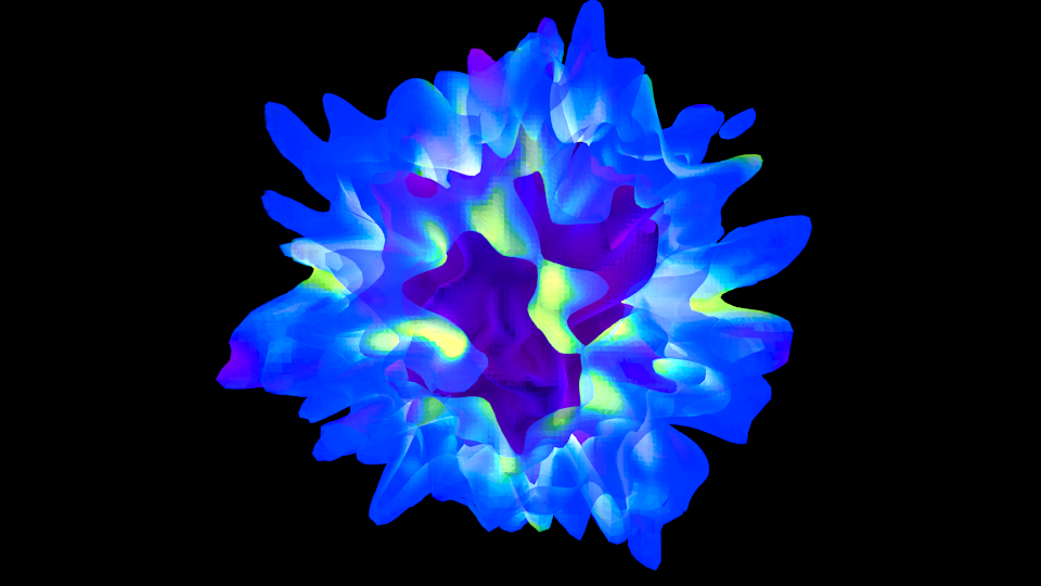
Note that the hottest stuff is brightly shining, while the cool stuff is less so (making the inner isodensity contour barely visible from the outside of the surfaces).

If the Blender image caught your fancy, you’ll be happy to know there is a greater integration of Blender and yt in the works, so stay tuned!