Unstructured Mesh Rendering

Beginning with version 3.3, yt has the ability to volume render unstructured mesh data like that created by finite element calculations. No additional dependencies are required in order to use this feature. However, it is possible to speed up the rendering operation by installing with Embree support. Embree is a fast ray-tracing library from Intel that can substantially speed up the mesh rendering operation on large datasets. You can read about how to install yt with Embree support below, or you can skip to the examples.

Optional Embree Installation

You’ll need to install Python bindings for netCDF4. Then you’ll need to get Embree itself and its corresponding Python bindings (pyembree). For conda-based systems, this is trivial, see pyembree’s doc

For systems other than conda, you will need to install Embree first, either by compiling from source or by using one of the pre-built binaries available at Embree’s releases page.

Then you’ll want to install pyembree from source as follows.

git clone https://github.com/scopatz/pyembree

To install, navigate to the root directory and run the setup script. If Embree was installed to some location that is not in your path by default, you will need to pass in CFLAGS and LDFLAGS to the setup.py script. For example, the Mac OS X package installer puts the installation at /opt/local/ instead of usr/local. To account for this, you would do:

CFLAGS='-I/opt/local/include' LDFLAGS='-L/opt/local/lib' python setup.py install

Once Embree and pyembree are installed, a,d in order to use the unstructured mesh rendering capability, you must rebuild yt from source, . Once again, if embree is installed in a location that is not part of your default search path, you must tell yt where to find it. There are a number of ways to do this. One way is to again manually pass in the flags when running the setup script in the yt-git directory:

CFLAGS='-I/opt/local/include' LDFLAGS='-L/opt/local/lib' python setup.py develop

You can also set EMBREE_DIR environment variable to ‘/opt/local’, in which case you could just run

python setup.py develop

as usual. Finally, if you create a file called embree.cfg in the yt-git directory with the location of the embree installation, the setup script will find this and use it, provided EMBREE_DIR is not set. An example embree.cfg file could like this:

/opt/local/

We recommend one of the later two methods, especially if you plan on re-compiling the cython extensions regularly. Note that none of this is necessary if you installed embree into a location that is in your default path, such as /usr/local.

Examples

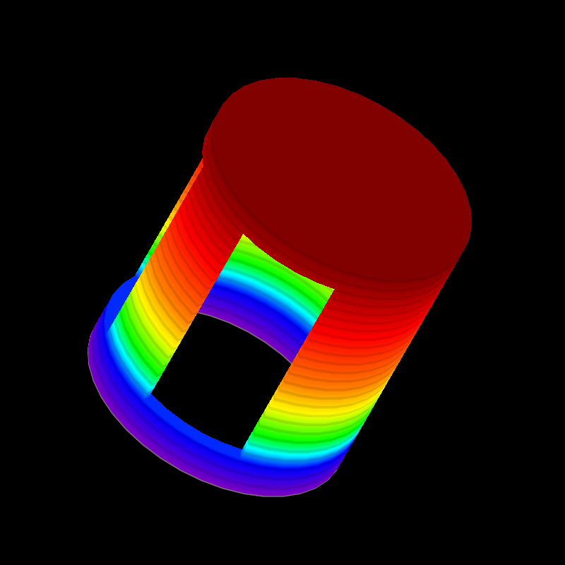
First, here is an example of rendering an 8-node, hexahedral MOOSE dataset.

import yt

ds = yt.load("MOOSE_sample_data/out.e-s010")

# create a default scene
sc = yt.create_scene(ds)

# override the default colormap
ms = sc.get_source()
ms.cmap = "Eos A"

# adjust the camera position and orientation
cam = sc.camera
cam.focus = ds.arr([0.0, 0.0, 0.0], "code_length")
cam_pos = ds.arr([-3.0, 3.0, -3.0], "code_length")
north_vector = ds.arr([0.0, -1.0, -1.0], "dimensionless")
cam.set_position(cam_pos, north_vector)

# increase the default resolution
cam.resolution = (800, 800)

# render and save
sc.save()

You can also overplot the mesh boundaries:

import yt

ds = yt.load("MOOSE_sample_data/out.e-s010")

# create a default scene
sc = yt.create_scene(ds)

# override the default colormap
ms = sc.get_source()
ms.cmap = "Eos A"

# adjust the camera position and orientation
cam = sc.camera
cam.focus = ds.arr([0.0, 0.0, 0.0], "code_length")
cam_pos = ds.arr([-3.0, 3.0, -3.0], "code_length")
north_vector = ds.arr([0.0, -1.0, -1.0], "dimensionless")
cam.set_position(cam_pos, north_vector)

# increase the default resolution
cam.resolution = (800, 800)

# render, draw the element boundaries, and save
sc.render()
sc.annotate_mesh_lines()
sc.save()

As with slices, you can visualize different meshes and different fields. For example, Here is a script similar to the above that plots the “diffused” variable using the mesh labelled by “connect2”:

import yt

ds = yt.load("MOOSE_sample_data/out.e-s010")

# create a default scene
sc = yt.create_scene(ds, ("connect2", "diffused"))

# override the default colormap
ms = sc.get_source()
ms.cmap = "Eos A"

# adjust the camera position and orientation
cam = sc.camera
cam.focus = ds.arr([0.0, 0.0, 0.0], "code_length")
cam_pos = ds.arr([-3.0, 3.0, -3.0], "code_length")
north_vector = ds.arr([0.0, -1.0, -1.0], "dimensionless")
cam.set_position(cam_pos, north_vector)

# increase the default resolution
cam.resolution = (800, 800)

# render and save
sc.save()

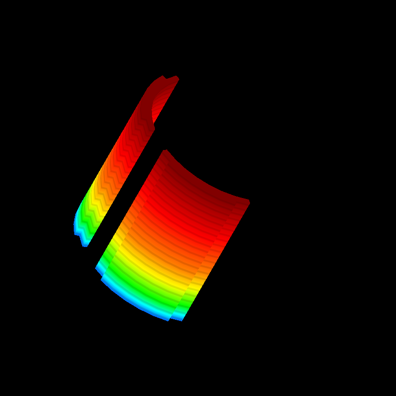
Next, here is an example of rendering a dataset with tetrahedral mesh elements. Note that in this dataset, there are multiple “steps” per file, so we specify that we want to look at the last one.

import yt

filename = "MOOSE_sample_data/high_order_elems_tet4_refine_out.e"
ds = yt.load(filename, step=-1)  # we look at the last time frame

# create a default scene
sc = yt.create_scene(ds, ("connect1", "u"))

# override the default colormap
ms = sc.get_source()
ms.cmap = "Eos A"

# adjust the camera position and orientation
cam = sc.camera
camera_position = ds.arr([3.0, 3.0, 3.0], "code_length")
cam.set_width(ds.arr([2.0, 2.0, 2.0], "code_length"))
north_vector = ds.arr([0.0, -1.0, 0.0], "dimensionless")
cam.set_position(camera_position, north_vector)

# increase the default resolution
cam.resolution = (800, 800)

# render and save
sc.save()

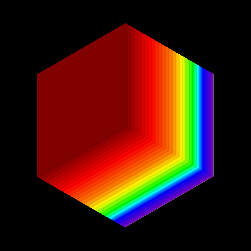
Here is an example using 6-node wedge elements:

import yt

ds = yt.load("MOOSE_sample_data/wedge_out.e")

# create a default scene
sc = yt.create_scene(ds, ("connect2", "diffused"))

# override the default colormap
ms = sc.get_source()
ms.cmap = "Eos A"

# adjust the camera position and orientation
cam = sc.camera
cam.set_position(ds.arr([1.0, -1.0, 1.0], "code_length"))
cam.width = ds.arr([1.5, 1.5, 1.5], "code_length")

# render and save
sc.save()

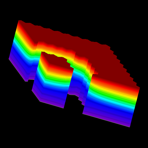
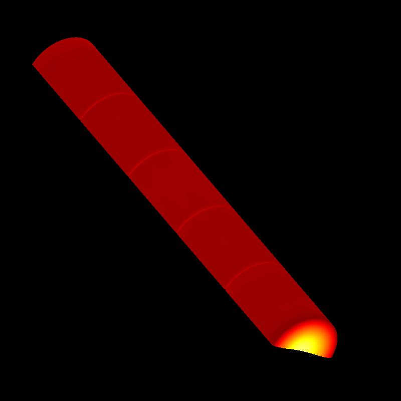
Another example, this time plotting the temperature field from a 20-node hex MOOSE dataset:

import yt

# We load the last time frame
ds = yt.load("MOOSE_sample_data/mps_out.e", step=-1)

# create a default scene
sc = yt.create_scene(ds, ("connect2", "temp"))

# override the default colormap. This time we also override
# the default color bounds
ms = sc.get_source()
ms.cmap = "hot"
ms.color_bounds = (500.0, 1700.0)

# adjust the camera position and orientation
cam = sc.camera
camera_position = ds.arr([-1.0, 1.0, -0.5], "code_length")
north_vector = ds.arr([0.0, -1.0, -1.0], "dimensionless")
cam.width = ds.arr([0.04, 0.04, 0.04], "code_length")
cam.set_position(camera_position, north_vector)

# increase the default resolution
cam.resolution = (800, 800)

# render, draw the element boundaries, and save
sc.render()
sc.annotate_mesh_lines()
sc.save()

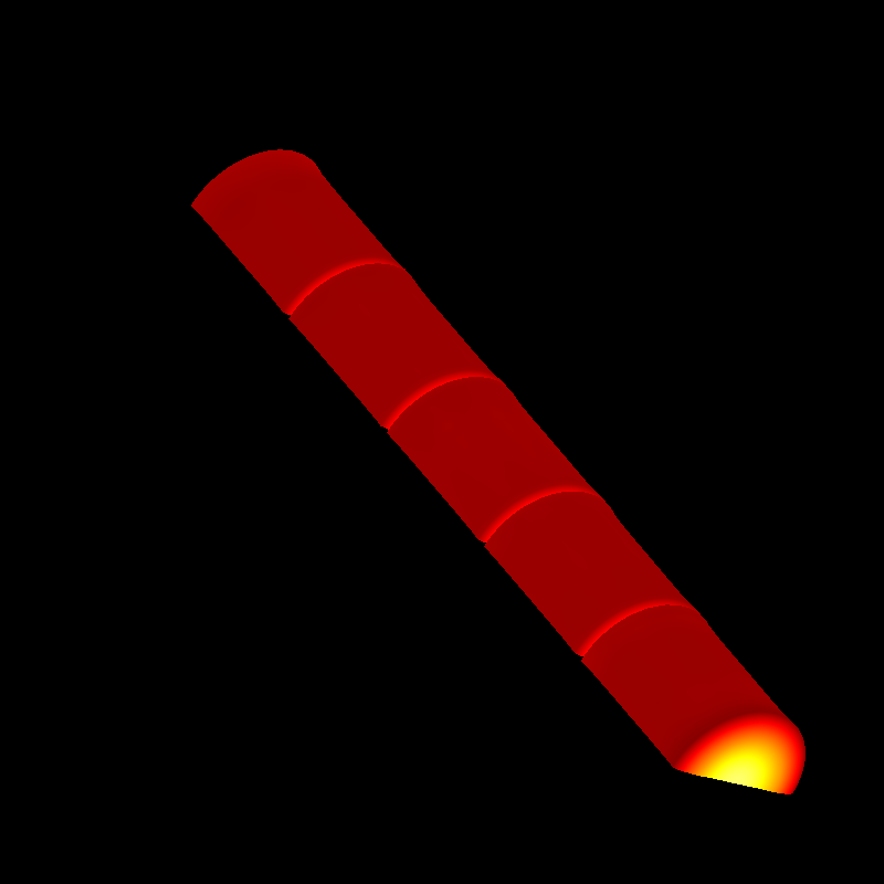
The dataset in the above example contains displacement fields, so this is a good opportunity to demonstrate their use. The following example is exactly like the above, except we scale the displacements by a factor of a 10.0, and additionally add an offset to the mesh by 1.0 unit in the x-direction:

import yt

# We load the last time frame
ds = yt.load(
    "MOOSE_sample_data/mps_out.e",
    step=-1,
    displacements={"connect2": (10.0, [0.01, 0.0, 0.0])},
)

# create a default scene
sc = yt.create_scene(ds, ("connect2", "temp"))

# override the default colormap. This time we also override
# the default color bounds
ms = sc.get_source()
ms.cmap = "hot"
ms.color_bounds = (500.0, 1700.0)

# adjust the camera position and orientation
cam = sc.camera
camera_position = ds.arr([-1.0, 1.0, -0.5], "code_length")
north_vector = ds.arr([0.0, -1.0, -1.0], "dimensionless")
cam.width = ds.arr([0.05, 0.05, 0.05], "code_length")
cam.set_position(camera_position, north_vector)

# increase the default resolution
cam.resolution = (800, 800)

# render, draw the element boundaries, and save
sc.render()
sc.annotate_mesh_lines()
sc.save()

As with other volume renderings in yt, you can swap out different lenses. Here is an example that uses a “perspective” lens, for which the rays diverge from the camera position according to some opening angle:

import yt

ds = yt.load("MOOSE_sample_data/out.e-s010")

# create a default scene
sc = yt.create_scene(ds, ("connect2", "diffused"))

# override the default colormap
ms = sc.get_source()
ms.cmap = "Eos A"

# Create a perspective Camera
cam = sc.add_camera(ds, lens_type="perspective")
cam.focus = ds.arr([0.0, 0.0, 0.0], "code_length")
cam_pos = ds.arr([-4.5, 4.5, -4.5], "code_length")
north_vector = ds.arr([0.0, -1.0, -1.0], "dimensionless")
cam.set_position(cam_pos, north_vector)

# increase the default resolution
cam.resolution = (800, 800)

# render, draw the element boundaries, and save
sc.render()
sc.annotate_mesh_lines()
sc.save()

You can also create scenes that have multiple meshes. The ray-tracing infrastructure will keep track of the depth information for each source separately, and composite the final image accordingly. In the next example, we show how to render a scene with two meshes on it:

import yt
from yt.visualization.volume_rendering.api import MeshSource, Scene

ds = yt.load("MOOSE_sample_data/out.e-s010")

# this time we create an empty scene and add sources to it one-by-one
sc = Scene()

# set up our Camera
cam = sc.add_camera(ds)
cam.focus = ds.arr([0.0, 0.0, 0.0], "code_length")
cam.set_position(
    ds.arr([-3.0, 3.0, -3.0], "code_length"),
    ds.arr([0.0, -1.0, 0.0], "dimensionless"),
)
cam.set_width = ds.arr([8.0, 8.0, 8.0], "code_length")
cam.resolution = (800, 800)

# create two distinct MeshSources from 'connect1' and 'connect2'
ms1 = MeshSource(ds, ("connect1", "diffused"))
ms2 = MeshSource(ds, ("connect2", "diffused"))

sc.add_source(ms1)
sc.add_source(ms2)

# render and save
im = sc.render()
sc.save()

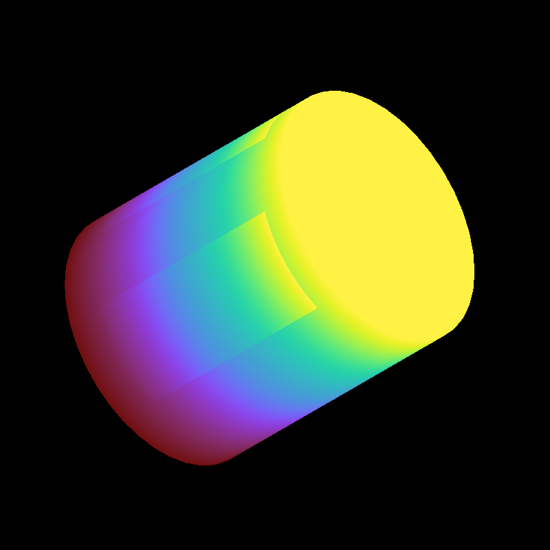
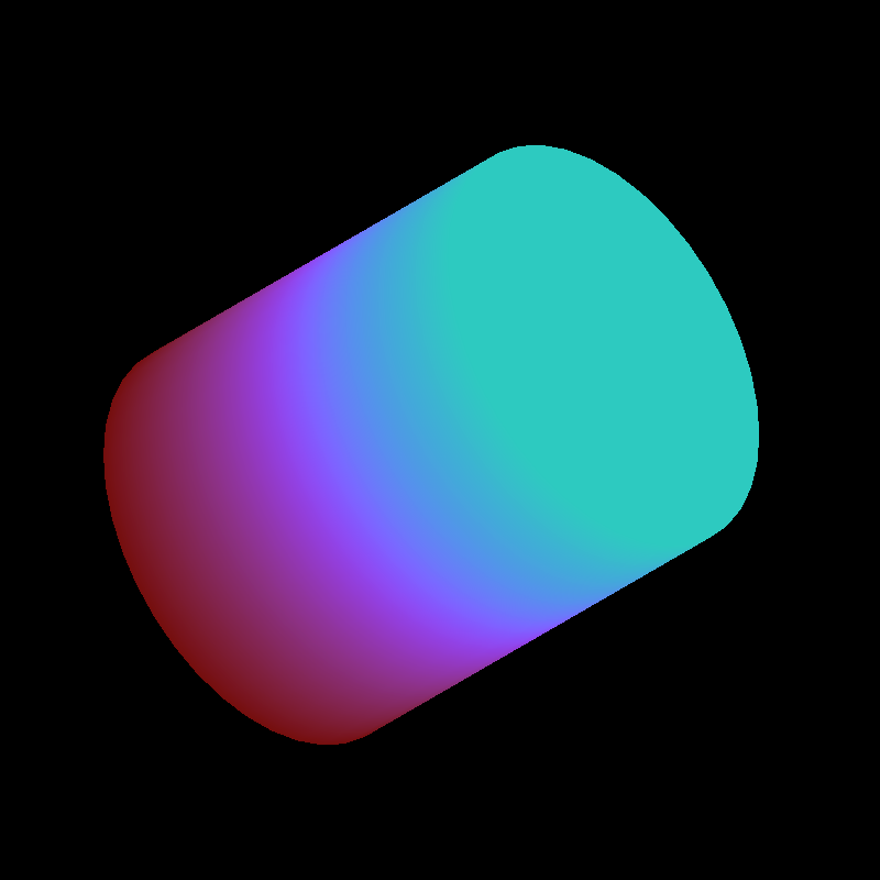
However, in the rendered image above, we note that the color is discontinuous on in the middle and upper part of the cylinder’s side. In the original data, there are two parts but the value of diffused is continuous at the interface. This discontinuous color is due to an independent colormap setting for the two mesh sources. To fix it, we can explicitly specify the colormap bound for each mesh source as follows:

import yt
from yt.visualization.volume_rendering.api import MeshSource, Scene

ds = yt.load("MOOSE_sample_data/out.e-s010")

# this time we create an empty scene and add sources to it one-by-one
sc = Scene()

# set up our Camera
cam = sc.add_camera(ds)
cam.focus = ds.arr([0.0, 0.0, 0.0], "code_length")
cam.set_position(
    ds.arr([-3.0, 3.0, -3.0], "code_length"),
    ds.arr([0.0, -1.0, 0.0], "dimensionless"),
)
cam.set_width = ds.arr([8.0, 8.0, 8.0], "code_length")
cam.resolution = (800, 800)

# create two distinct MeshSources from 'connect1' and 'connect2'
ms1 = MeshSource(ds, ("connect1", "diffused"))
ms2 = MeshSource(ds, ("connect2", "diffused"))

# add the following lines to set the range of the two mesh sources
ms1.color_bounds = (0.0, 3.0)
ms2.color_bounds = (0.0, 3.0)

sc.add_source(ms1)
sc.add_source(ms2)

# render and save
im = sc.render()
sc.save()

Making Movies

Here are a couple of example scripts that show how to create image frames that can later be stitched together into a movie. In the first example, we look at a single dataset at a fixed time, but we move the camera around to get a different vantage point. We call the rotate() method 300 times, saving a new image to the disk each time.

import numpy as np

import yt

ds = yt.load("MOOSE_sample_data/out.e-s010")

# create a default scene
sc = yt.create_scene(ds)

# override the default colormap
ms = sc.get_source()
ms.cmap = "Eos A"

# adjust the camera position and orientation
cam = sc.camera
cam.focus = ds.arr([0.0, 0.0, 0.0], "code_length")
cam_pos = ds.arr([-3.0, 3.0, -3.0], "code_length")
north_vector = ds.arr([0.0, -1.0, -1.0], "dimensionless")
cam.set_position(cam_pos, north_vector)

# increase the default resolution
cam.resolution = (800, 800)

# set the camera to use "steady_north"
cam.steady_north = True

# make movie frames
num_frames = 301
for i in range(num_frames):
    cam.rotate(2.0 * np.pi / num_frames)
    sc.render()
    sc.save("movie_frames/surface_render_%.4d.png" % i)

Finally, this example demonstrates how to loop over the time steps in a single file with a fixed camera position:

import matplotlib.pyplot as plt

import yt
from yt.visualization.volume_rendering.api import MeshSource

NUM_STEPS = 127
CMAP = "hot"
VMIN = 300.0
VMAX = 2000.0

for step in range(NUM_STEPS):
    ds = yt.load("MOOSE_sample_data/mps_out.e", step=step)

    time = ds._get_current_time()

    # the field name is a tuple of strings. The first string
    # specifies which mesh will be plotted, the second string
    # specifies the name of the field.
    field_name = ('connect2', 'temp')

    # this initializes the render source
    ms = MeshSource(ds, field_name)

    # set up the camera here. these values were arrived by
    # calling pitch, yaw, and roll in the notebook until I
    # got the angle I wanted.
    sc.add_camera(ds)
    camera_position = ds.arr([0.1, 0.0, 0.1], 'code_length')
    cam.focus = ds.domain_center
    north_vector = ds.arr([-0.3032476, -0.71782557, 0.62671153], 'dimensionless')
    cam.width = ds.arr([ 0.04,  0.04,  0.04], 'code_length')
    cam.resolution = (800, 800)
    cam.set_position(camera_position, north_vector)

    # actually make the image here
    im = ms.render(cam, cmap=CMAP, color_bounds=(VMIN, VMAX))

    # Plot the result using matplotlib and save.
    # Note that we are setting the upper and lower
    # bounds of the colorbar to be the same for all
    # frames of the image.

    # must clear the image between frames
    plt.clf()
    fig = plt.gcf()
    ax = plt.gca()
    ax.imshow(im, interpolation='nearest', origin='lower')

    # Add the colorbar using a fake (not shown) image.
    p = ax.imshow(ms.data, visible=False, cmap=CMAP, vmin=VMIN, vmax=VMAX)
    cb = fig.colorbar(p)
    cb.set_label(field_name[1])

    ax.text(25, 750, 'time = %.2e' % time, color='k')
    ax.axes.get_xaxis().set_visible(False)
    ax.axes.get_yaxis().set_visible(False)

    plt.savefig('movie_frames/test_%.3d' % step)