Using the Manual Plotting Interface¶

Sometimes you need a lot of flexibility in creating plots. While the PlotWindow provides an easy to use object that can create nice looking, publication quality plots with a minimum of effort, there are often times when its ease of use conflicts with your need to change the font only on the x-axis, or whatever your need/desire/annoying coauthor requires. To that end, yt provides a number of ways of getting the raw data that goes into a plot to you in the form of a one or two dimensional dataset that you can plot using any plotting method you like. matplotlib or another python library are easiest, but these methods allow you to take your data and plot it in gnuplot, or any unnamed commercial plotting packages.

Note that the index object associated with your snapshot file contains a list of plots you’ve made in ds.plots.

Slice, Projections, and other Images: The Fixed Resolution Buffer¶

For slices and projects, yt provides a manual plotting interface based on the FixedResolutionBuffer (hereafter referred to as FRB) object. Despite its somewhat unwieldy name, at its heart, an FRB is a very simple object: it’s essentially a window into your data: you give it a center and a width or a left and right edge, and an image resolution, and the FRB returns a fully pixelized image. The simplest way to generate an FRB is to use the .to_frb(width, resolution, center=None) method of any data two-dimensional data object:

import matplotlib

matplotlib.use("Agg")
import numpy as np
from matplotlib import pyplot as plt

import yt

ds = yt.load("IsolatedGalaxy/galaxy0030/galaxy0030")

_, c = ds.find_max(("gas", "density"))
proj = ds.proj(("gas", "density"), 0)

width = (10, "kpc")  # we want a 1.5 mpc view
res = [1000, 1000]  # create an image with 1000x1000 pixels
frb = proj.to_frb(width, res, center=c)

plt.imshow(np.array(frb["gas", "density"]))
plt.savefig("my_perfect_figure.png")

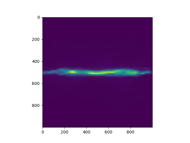
Note that in the above example the axes tick marks indicate pixel indices. If you want to represent physical distances on your plot axes, you will need to use the extent keyword of the imshow function.

The FRB is a very small object that can be deleted and recreated quickly (in fact, this is how PlotWindow plots work behind the scenes). Furthermore, you can add new fields in the same “window”, and each of them can be plotted with their own zlimit. This is quite useful for creating a mosaic of the same region in space with Density, Temperature, and x-velocity, for example. Each of these quantities requires a substantially different set of limits.

A more complex example, showing a few yt helper functions that can make setting up multiple axes with colorbars easier than it would be using only matplotlib can be found in the Advanced Multi-Plot Multi-Panel cookbook recipe.

Fixed Resolution Buffer Filters¶

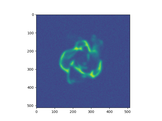
The FRB can be modified by using set of predefined filters in order to e.g. create realistically looking, mock observation images out of simulation data. Applying filter is an irreversible operation, hence the order in which you are using them matters.

import matplotlib

matplotlib.use("Agg")
from matplotlib import pyplot as plt

import yt

ds = yt.load("IsolatedGalaxy/galaxy0030/galaxy0030")
slc = ds.slice("z", 0.5)
frb = slc.to_frb((20, "kpc"), 512)
frb.apply_gauss_beam(nbeam=30, sigma=2.0)
frb.apply_white_noise(5e-23)
plt.imshow(frb["gas", "density"].d)
plt.savefig("frb_filters.png")

Currently available filters:

Gaussian Smoothing¶

apply_gauss_beam(self, nbeam=30, sigma=2.0)¶: (This is a proxy for FixedResolutionBufferGaussBeamFilter.)

This filter convolves the FRB with 2d Gaussian that is “nbeam” pixel wide and has standard deviation “sigma”.

White Noise¶

apply_white_noise(self, bg_lvl=None)¶: (This is a proxy for FixedResolutionBufferWhiteNoiseFilter.)

This filter adds white noise with the amplitude “bg_lvl” to the FRB. If “bg_lvl” is not present, 10th percentile of the FRB’s values is used instead.

Line Plots¶

This is perhaps the simplest thing to do. yt provides a number of one dimensional objects, and these return a 1-D numpy array of their contents with direct dictionary access. As a simple example, take a YTOrthoRay object, which can be created from a index by calling ds.ortho_ray(axis, center).

import matplotlib

matplotlib.use("Agg")
import numpy as np
from matplotlib import pyplot as plt

import yt

ds = yt.load("IsolatedGalaxy/galaxy0030/galaxy0030")
_, c = ds.find_max(("gas", "density"))
ax = 0  # take a line cut along the x axis

# cutting through the y0,z0 such that we hit the max density
ray = ds.ortho_ray(ax, (c[1], c[2]))

# Sort the ray values by 'x' so there are no discontinuities
# in the line plot
srt = np.argsort(ray["index", "x"])

plt.subplot(211)
plt.semilogy(np.array(ray["index", "x"][srt]), np.array(ray["gas", "density"][srt]))
plt.ylabel("density")
plt.subplot(212)
plt.semilogy(np.array(ray["index", "x"][srt]), np.array(ray["gas", "temperature"][srt]))
plt.xlabel("x")
plt.ylabel("temperature")

plt.savefig("den_temp_xsweep.png")

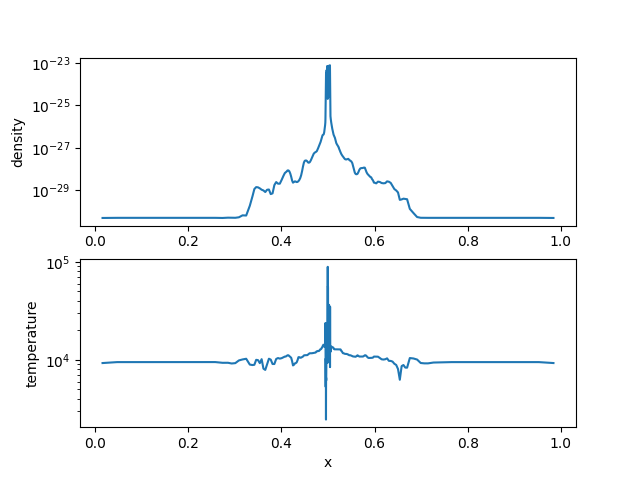
Of course, you’ll likely want to do something more sophisticated than using the matplotlib defaults, but this gives the general idea.