Streamlines: Tracking the Trajectories of Tracers in your Data

Streamlines, as implemented in yt, are defined as being parallel to a vector field at all points. While commonly used to follow the velocity flow or magnetic field lines, they can be defined to follow any three-dimensional vector field. Once an initial condition and total length of the streamline are specified, the streamline is uniquely defined. Relatedly, yt also has the ability to follow Particle Trajectories.

Method

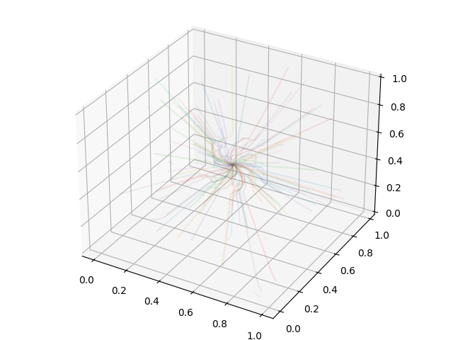
Streamlining through a volume is useful for a variety of analysis tasks. By specifying a set of starting positions, the user is returned a set of 3D positions that can, in turn, be used to visualize the 3D path of the streamlines. Additionally, individual streamlines can be converted into YTStreamline objects, and queried for all the available fields along the streamline.

The implementation of streamlining in yt is described below.

1. Decompose the volume into a set of non-overlapping, fully domain tiling bricks, using the AMRKDTree homogenized volume.

2. For every streamline starting position:

   1. While the length of the streamline is less than the requested length:

      1. Find the brick that contains the current position

      2. If not already present, generate vertex-centered data for the vector fields defining the streamline.

      3. While inside the brick

         1. Integrate the streamline path using a Runge-Kutta 4th order method and the vertex centered data.

         2. During the intermediate steps of each RK4 step, if the position is updated to outside the current brick, interrupt the integration and locate a new brick at the intermediate position.

3. The set of streamline positions are stored in the Streamlines object.

Example Script

import matplotlib.pyplot as plt
import numpy as np
from mpl_toolkits.mplot3d import Axes3D

import yt
from yt.units import Mpc
from yt.visualization.api import Streamlines

# Load the dataset
ds = yt.load("IsolatedGalaxy/galaxy0030/galaxy0030")

# Define c: the center of the box, N: the number of streamlines,
# scale: the spatial scale of the streamlines relative to the boxsize,
# and then pos: the random positions of the streamlines.
c = ds.domain_center
N = 100
scale = ds.domain_width[0]
pos_dx = np.random.random((N, 3)) * scale - scale / 2.0
pos = c + pos_dx

# Create streamlines of the 3D vector velocity and integrate them through
# the box defined above
streamlines = Streamlines(
    ds,
    pos,
    ("gas", "velocity_x"),
    ("gas", "velocity_y"),
    ("gas", "velocity_z"),
    length=1.0 * Mpc,
    get_magnitude=True,
)
streamlines.integrate_through_volume()

# Create a 3D plot, trace the streamlines through the 3D volume of the plot
fig = plt.figure()
ax = Axes3D(fig, auto_add_to_figure=False)
fig.add_axes(ax)
for stream in streamlines.streamlines:
    stream = stream[np.all(stream != 0.0, axis=1)]
    ax.plot3D(stream[:, 0], stream[:, 1], stream[:, 2], alpha=0.1)

# Save the plot to disk.
plt.savefig("streamlines.png")

Data Access Along the Streamline

Note

This functionality has not been implemented yet in the 3.x series of yt. If you are interested in working on this and have questions, please let us know on the yt-dev mailing list.

Once the streamlines are found, a YTStreamline object can be created using the path() function, which takes as input the index of the streamline requested. This conversion is done by creating a mask that defines where the streamline is, and creating ‘t’ and ‘dts’ fields that define the dimensionless streamline integration coordinate and integration step size. Once defined, fields can be accessed in the standard manner.

Example Script

import matplotlib.pyplot as plt
import yt
from yt.visualization.api import Streamlines

ds = yt.load("DD1701")  # Load ds
streamlines = Streamlines(ds, ds.domain_center)
streamlines.integrate_through_volume()
stream = streamlines.path(0)
plt.semilogy(stream["t"], stream["gas", "density"], "-x")

Running in Parallel

The integration of the streamline paths is “embarrassingly” parallelized by splitting the streamlines up between the processors. Upon completion, each processor has access to all of the streamlines through the use of a reduction operation.

For more information on enabling parallelism in yt, see Parallel Computation With yt.