Volume Rendering Tutorial

This notebook shows how to use the new (in version 3.3) Scene interface to create custom volume renderings. The tutorial proceeds in the following steps:

1. Creating the Scene

2. Displaying the Scene

3. Adjusting Transfer Functions

4. Saving an Image

5. Adding Annotations

1. Creating the Scene

To begin, we load up a dataset and use the yt.create_scene method to set up a basic Scene. We store the Scene in a variable called sc and render the default ('gas', 'density') field.

import yt
from yt.visualization.volume_rendering.transfer_function_helper import (
    TransferFunctionHelper,
)

ds = yt.load("IsolatedGalaxy/galaxy0030/galaxy0030")
sc = yt.create_scene(ds)

Note that to render a different field, we would use pass the field name to yt.create_scene using the field argument.

Now we can look at some information about the Scene we just created using the python print keyword:

print(sc)

<Scene Object>:
Sources:
    source_00: <Volume Source>:YTRegion (galaxy0030): , center=[1.543e+24 1.543e+24 1.543e+24] cm, left_edge=[0. 0. 0.] cm, right_edge=[3.086e+24 3.086e+24 3.086e+24] cm transfer_function:None
Camera:
    <Camera Object>:
        position:[1. 1. 1.] code_length
        focus:[0.5 0.5 0.5] code_length
        north_vector:[ 0.81649658 -0.40824829 -0.40824829] dimensionless
        width:[1.5 1.5 1.5] code_length
        light:None
        resolution:(512, 512)
Lens: <Lens Object>:
        lens_type:plane-parallel
        viewpoint:[-866025.33679714 -866025.33679714 -866025.33679714] code_length

This prints out information about the Sources, Camera, and Lens associated with this Scene. Each of these can also be printed individually. For example, to print only the information about the first (and currently, only) Source, we can do:

print(sc.get_source())

<Volume Source>:YTRegion (galaxy0030): , center=[1.543e+24 1.543e+24 1.543e+24] cm, left_edge=[0. 0. 0.] cm, right_edge=[3.086e+24 3.086e+24 3.086e+24] cm transfer_function:None

2. Displaying the Scene

We can see that the yt.create_source method has created a VolumeSource with default values for the center, bounds, and transfer function. Now, let’s see what this Scene looks like. In the notebook, we can do this by calling sc.show().

sc.show()

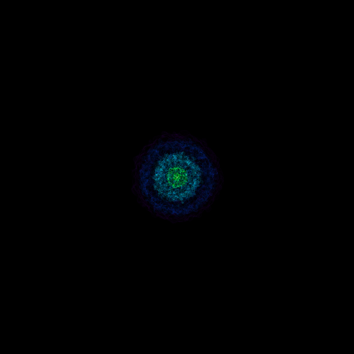
That looks okay, but it’s a little too zoomed-out. To fix this, let’s modify the Camera associated with our Scene. This next bit of code will zoom in the camera (i.e. decrease the width of the view) by a factor of 3.

sc.camera.zoom(3.0)

Now when we print the Scene, we see that the Camera width has decreased by a factor of 3:

print(sc)

<Scene Object>:
Sources:
    source_00: <Volume Source>:YTRegion (galaxy0030): , center=[1.543e+24 1.543e+24 1.543e+24] cm, left_edge=[0. 0. 0.] cm, right_edge=[3.086e+24 3.086e+24 3.086e+24] cm transfer_function:<Color Transfer Function Object>:
x_bounds:[-31, -23] nbins:512 features:
        ('gaussian', 'location(x):-31', 'width(x):0.002', 'height(y):(0.073,   0, 0.084, 0.001)')
        ('gaussian', 'location(x):-30', 'width(x):0.002', 'height(y):(0.35,   0, 0.62, 0.0022)')
        ('gaussian', 'location(x):-29', 'width(x):0.002', 'height(y):(  0, 0.26, 0.87, 0.0046)')
        ('gaussian', 'location(x):-28', 'width(x):0.002', 'height(y):(  0, 0.65, 0.72, 0.01)')
        ('gaussian', 'location(x):-28', 'width(x):0.002', 'height(y):(  0, 0.6, 0.031, 0.022)')
        ('gaussian', 'location(x):-27', 'width(x):0.002', 'height(y):(  0, 0.87,   0, 0.046)')
        ('gaussian', 'location(x):-26', 'width(x):0.002', 'height(y):(0.78, 0.98,   0, 0.1)')
        ('gaussian', 'location(x):-25', 'width(x):0.002', 'height(y):(  1, 0.71,   0, 0.22)')
        ('gaussian', 'location(x):-24', 'width(x):0.002', 'height(y):(0.91,   0,   0, 0.46)')
        ('gaussian', 'location(x):-23', 'width(x):0.002', 'height(y):(0.8, 0.67, 0.67,   1)')

Camera:
    <Camera Object>:
        position:[1. 1. 1.] code_length
        focus:[0.5 0.5 0.5] code_length
        north_vector:[ 0.81649658 -0.40824829 -0.40824829] dimensionless
        width:[0.5 0.5 1.5] code_length
        light:None
        resolution:(512, 512)
Lens: <Lens Object>:
        lens_type:plane-parallel
        viewpoint:[-866025.33679714 -866025.33679714 -866025.33679714] code_length

To see what this looks like, we re-render the image and display the scene again. Note that we don’t actually have to call sc.show() here - we can just have Ipython evaluate the Scene and that will display it automatically.

sc.render()
sc

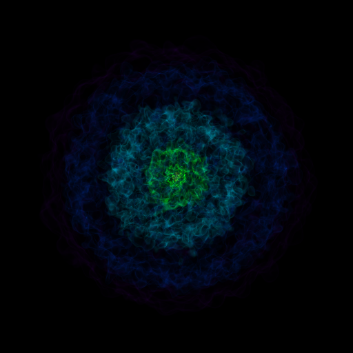
That’s better! The image looks a little washed-out though, so we use the sigma_clip argument to sc.show() to improve the contrast:

sc.show(sigma_clip=4.0)

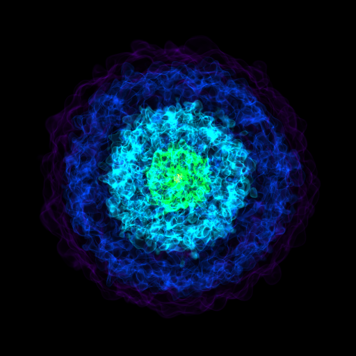
Applying different values of sigma_clip with sc.show() is a relatively fast process because sc.show() will pull the most recently rendered image and apply the contrast adjustment without rendering the scene again. While this is useful for quickly testing the affect of different values of sigma_clip, it can lead to confusion if we don’t remember to render after making changes to the camera. For example, if we zoom in again and simply call sc.show(), then we get the same image as before:

sc.camera.zoom(3.0)
sc.show(sigma_clip=4.0)

For the change to the camera to take affect, we have to explicitly render again:

sc.render()
sc.show(sigma_clip=4.0)

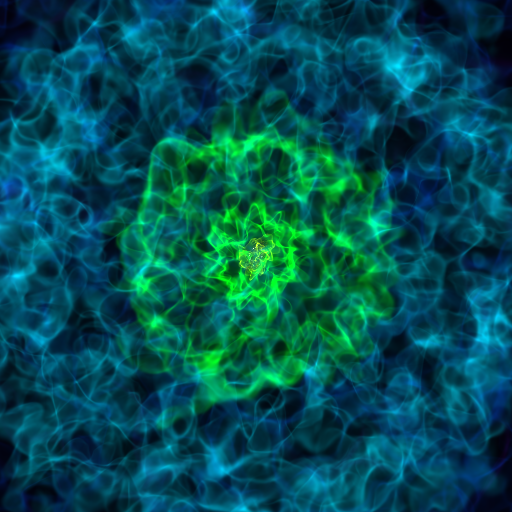
As a general rule, any changes to the scene itself such as adjusting the camera or changing transfer functions requires rendering again. Before moving on, let’s undo the last zoom:

sc.camera.zoom(1.0 / 3.0)

3. Adjusting Transfer Functions

Next, we demonstrate how to change the mapping between the field values and the colors in the image. We use the TransferFunctionHelper to create a new transfer function using the gist_rainbow colormap, and then re-create the image as follows:

# Set up a custom transfer function using the TransferFunctionHelper.
# We use 10 Gaussians evenly spaced logarithmically between the min and max
# field values.
tfh = TransferFunctionHelper(ds)
tfh.set_field("density")
tfh.set_log(True)
tfh.set_bounds()
tfh.build_transfer_function()
tfh.tf.add_layers(10, colormap="gist_rainbow")

# Grab the first render source and set it to use the new transfer function
render_source = sc.get_source()
render_source.transfer_function = tfh.tf

sc.render()
sc.show(sigma_clip=4.0)

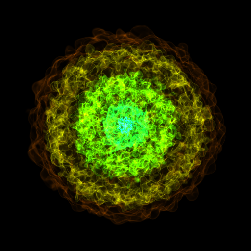
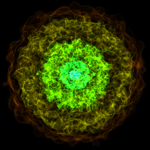
Now, let’s try using a different lens type. We can give a sense of depth to the image by using the perspective lens. To do, we create a new Camera below. We also demonstrate how to switch the camera to a new position and orientation.

cam = sc.add_camera(ds, lens_type="perspective")

# Standing at (x=0.05, y=0.5, z=0.5), we look at the area of x>0.05 (with some open angle
# specified by camera width) along the positive x direction.
cam.position = ds.arr([0.05, 0.5, 0.5], "code_length")

normal_vector = [1.0, 0.0, 0.0]
north_vector = [0.0, 0.0, 1.0]
cam.switch_orientation(normal_vector=normal_vector, north_vector=north_vector)

# The width determines the opening angle
cam.set_width(ds.domain_width * 0.5)

print(sc.camera)

<Camera Object>:
        position:[0.05 0.5  0.5 ] unitary
        focus:[0.5 0.5 0.5] code_length
        north_vector:[0. 0. 1.] dimensionless
        width:[0.5 0.5 0.5] unitary
        light:None
        resolution:(512, 512)
Lens: <Lens Object>:
        lens_type:perspective
        viewpoint:[0.75 0.5  0.5 ] code_length

The resulting image looks like:

sc.render()
sc.show(sigma_clip=4.0)

4. Saving an Image

To save a volume rendering to an image file at any point, we can use sc.save as follows:

sc.save("volume_render.png", render=False)

Including the keyword argument render=False indicates that the most recently rendered image will be saved (otherwise, sc.save() will trigger a call to sc.render()). This behavior differs from sc.show(), which always uses the most recently rendered image.

An additional caveat is that if we used sigma_clip in our call to sc.show(), then we must also pass it to sc.save() as sigma clipping is applied on top of a rendered image array. In that case, we would do the following:

sc.save("volume_render_clip4.png", sigma_clip=4.0, render=False)

5. Adding Annotations

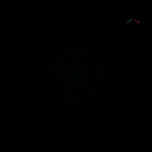
Finally, the next cell restores the lens and the transfer function to the defaults, moves the camera, and adds an opaque source that shows the axes of the simulation coordinate system.

# set the lens type back to plane-parallel
sc.camera.set_lens("plane-parallel")

# move the camera to the left edge of the domain
sc.camera.set_position(ds.domain_left_edge)
sc.camera.switch_orientation()

# add an opaque source to the scene
sc.annotate_axes()

sc.render()
sc.show(sigma_clip=4.0)