This presentaion is available at the following URL as slides and a Jupyter notebook at the following URLs:
http://yt-project.org/pitp2016_demo/yt_tutorial.slides.html
http://yt-project.org/pitp2016_demo/yt_tutorial.ipynb
The data I use in this presentation are available at the following URL:
http://yt-project.org/pitp2016_demo/data
The example notebooks I'll be working through in a focus session are available here:
yt is a framework for working with the ouputs of simulation codes
visualization
- slices
- projections
- volume rendering
- phase diagrams
analysis
- data selection and derived quantities
- low-level data inspection
- profiling (how does a quantity vary with radius? density?)
- and much more...
yt supports many production astrophysical simulation codes
- SPH (Gadget, Gasoline, Tipsy, ...)
- Patch AMR (Enzo, Athena, Chombo, ...)
- Octree AMR (FLASH, ART, ...)
- Unstructured Mesh (Moab, Exodus II, ...)
yt runs on a variety of platforms
- Operating systems: Linux, macOS, Windows (including the new Bash on Windows!)
- Runs on everything from laptops (e.g., this one) to supercomputers (e.g., NASA's Pleiades)
- Currently runs in Python 2.7 and 3.5
- Source installs and binaries are available
Developed by a global team of astrophysics researchers to solve their real-world problems.
| Tom Abel | Andrew Cunningham | Cameron Hummels | Michael Kuhlen | Desika Narayanan | Hsi-Yu Schive | Ting-Wai To |
| Gabriel Altay | Bili Dong | Suoqing Ji | Meagan Lang | Kaylea Nelson | Anthony Scopatz | Joseph Tomlinson |
| Kenza Arraki | Nicholas Earl | Allyson Julian | Eve Lee | Brian O'Shea | Noel Scudder | Stephanie Tonnesen |
| Kirk Barrow | Hilary Egan | Anni Järvenpää | Doris Lee | J.S. Oishi | Sam Skillman | Matthew Turk |
| Ricarda Beckmann | Rasmi Elasmar | Christian Karch | Sam Leitner | JC Passy | Stephen Skory | Casey W. Stark |
| Elliott Biondo | Daniel Fenn | Max Katz | Stuart Levy | John Regan | Aaron Smith | Miguel de Val-Borro |
| Alex Bogert | John Forbes | BW Keller | Yuan Li | Mark Richardson | Britton Smith | Rick Wagner |
| Robert Bradshaw | Sam Geen | Ji-hoon Kim | Joshua Moloney | Sherwood Richers | Geoffrey So | Mike Warren |
| Yi-Hao Chen | Adam Ginsburg | Steffen Klemer | Christopher Moody | Thomas Robitaille | Antoine Strugarek | Andrew Wetzel |
| Pengfei Chen | Nathan Goldbaum | Fabian Koller | Stuart Mumford | Anna Rosen | Elizabeth Tasker | John Wise |
| David Collins | Eric Hallman | Kacper Kowalik | Andrew Myers | Chuck Rozhon | Benjamin Thompson | Michael Zingale |
| Brian Crosby | David Hannasch | Mark Krumholz | Jill Naiman | Douglas Rudd | Robert Thompson | John ZuHone |
from __future__ import print_function
import warnings
warnings.filterwarnings('ignore')
from IPython.display import IFrame
IFrame('http://yt-project.org/docs/dev/reference/code_support.html', width=960, height=600)
Sample datasets loadable by yt
IFrame('http://yt-project.org/data', width=700, height=500)
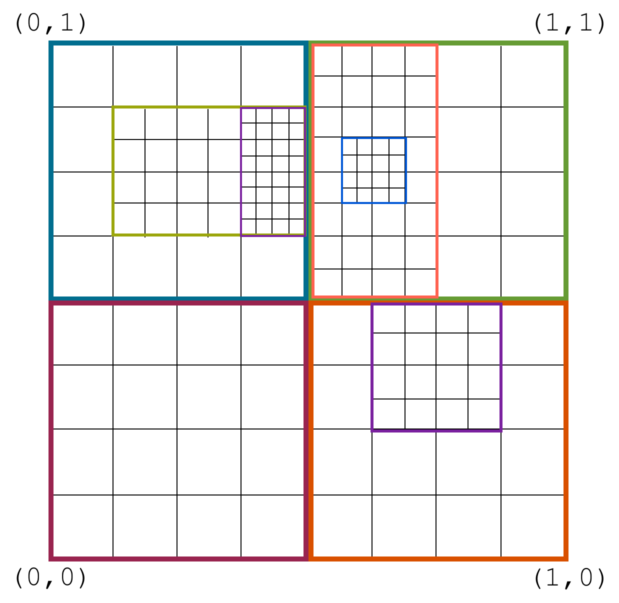
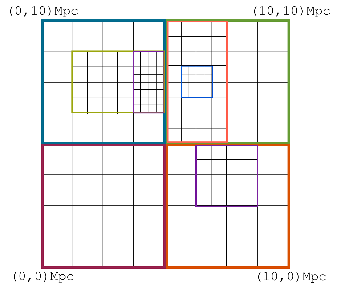
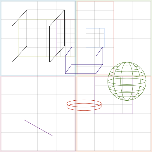
Eulerian, gridded, AMR/SMR data vs. Lagrangian, particle-based, SPH data
Data on disk has no inherent physical meaning
yt lets you think about the data using a physically motivated interface
- Data Objects
- Fields
- Units
- Derived Quantities
yt lets you think about the data using a physically motivated interface
import yt
ds = yt.load('data/DD0046/DD0046')
Allowing you to forget about what your data looks like as a file format
And select only the data you want to select

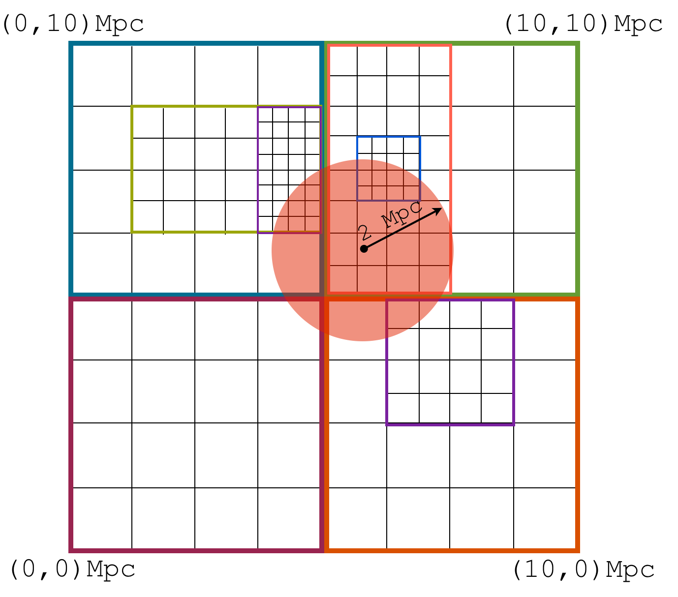
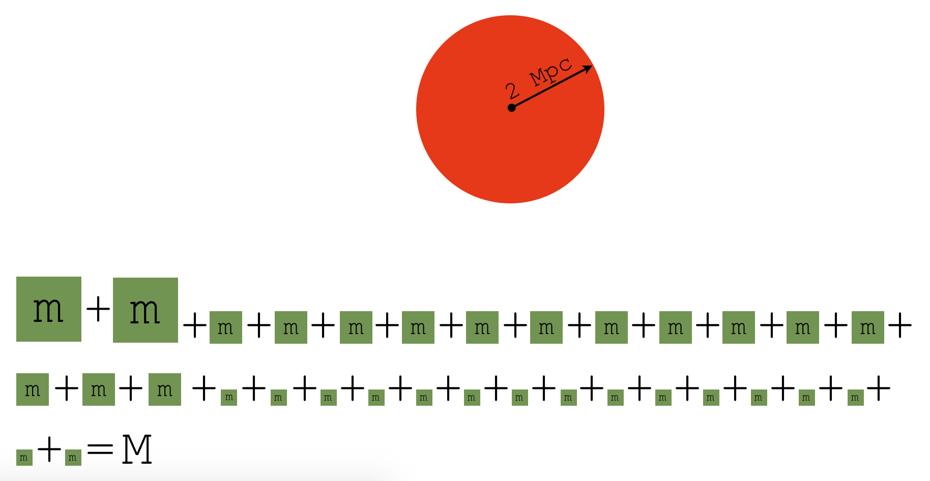
Data Objects
Physical objects to select data are called "data objects"

sp = ds.sphere("max", (2.0, "Mpc"))
yt natively deals with multiresolution data

Data from each selected cell is returned as a flat, 1D array, with unit metadata attached

print(sp['density'])
Data objects can be queried for many fields
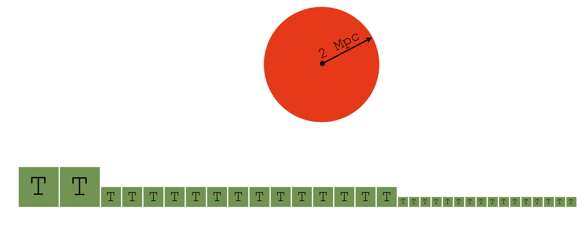
print(sp['temperature'])
Spatial information is not lost

sp['x']
sp['x'].in_units('kpc')
Spatial information is not lost
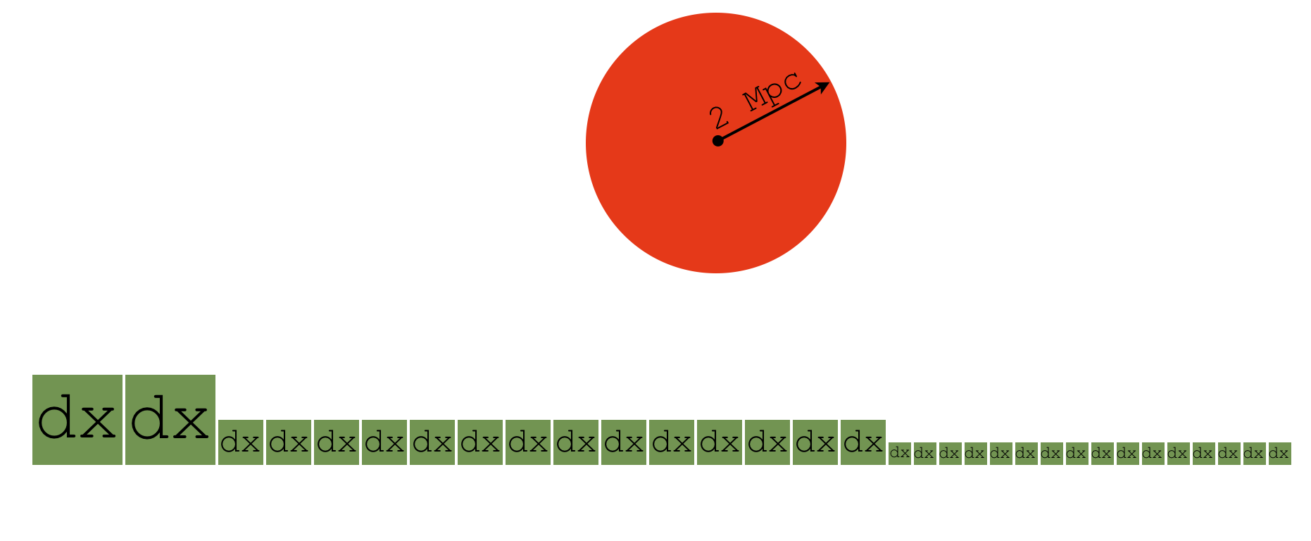
import numpy as np
np.unique(sp['dx']).in_units('kpc')
IFrame("http://yt-project.org/doc/analyzing/objects.html#available-objects", width=700, height=600)
import yt.units as u
ad = ds.all_data()
box = ds.box(ds.domain_left_edge + 500*u.kpc, ds.domain_right_edge - 500*u.kpc)
sp = ds.sphere(ds.domain_center, 500*u.kpc)
disk = ds.disk(ds.domain_center, [0, 0, 1], 500*u.kpc, 100*u.kpc)
ray = ds.ray(ds.domain_left_edge, ds.domain_right_edge)
Fields
Data objects can be queried for many fields
from pprint import pprint
# fields that are defined in the on-disk data file
pprint(ds.field_list)
Data objects can be queried for many fields
# fields that yt can calculate given the fields in ds.field_list
# (only showing gas fields to fit on one screen)
pprint([f for f in ds.derived_field_list if f[0]=='gas'][:20])
Particle fields
pprint([f for f in ds.field_list if f[0]=='io'])
ad = ds.all_data()
print(ad['io', 'particle_position'])
print(ad['io', 'particle_mass'])
Deposit Fields
pprint([f for f in ds.derived_field_list if f[0]=='deposit'])
Derived Fields: create new fields by defining a python function
from yt.units import kboltz, mh
def my_entropy(field, data):
return (kboltz * data['temperature'] / data['number_density']**(2./3.))
ds.add_field('entropy', function=my_entropy, units="keV*cm**2")
Derived Fields: create new fields by defining a python function

sp['entropy']
yt employs a field "democracy"
- Fields on-disk and derived fields are treated in exactly the same way
- Accessed the same way, visualized the same way
- On-disk fields are mapped to a set of common fields, to faciliate using the same scripts across different datasets
print(sp["gas","density"])
print(sp["enzo","Density"]) # These are the same field, just aliased
print(sp["enzo","Density"].in_cgs())
Units
We've already seen how data objects return fields as unit-aware NumPy arrays

pressure = sp['density']*sp['temperature']*kboltz/(0.6*mh)
pressure.in_units('Pa')
pressure.in_units('dyne/cm**2')
yt has very flexible handling for units and unit conversions
rho = sp['density']
print (rho.in_units('g/cm**3'))
print ()
print (rho.in_units('Msun/kpc**3'))
print ()
print (rho.in_units('code_mass/code_length**3')) # What's this?
Shorthand conversions for different unit systems
# Methods for MKSA and cgs/Gaussian units
print(rho.in_mks())
print()
print(rho.in_cgs())
Other unit systems are available
print(list(yt.unit_system_registry.keys()))
yt.unit_system_registry['mks']
Let's look at some of the unit systems
yt.unit_system_registry['imperial']
yt.unit_system_registry['geometrized']
We can convert into these other systems, too
print(rho.in_base('imperial'))
print()
print(rho.in_base('galactic'))
print()
print(rho.in_base('geometrized'))
But don't do something silly!
T = sp['temperature']
T.convert_to_units('kpc') # oops
You can also make your own unitful arrays, and quantities too
from yt import YTArray, YTQuantity
a = YTArray(np.random.random(10), "kpc")
print(a)
b = YTQuantity(1.0e-27, "erg/s/cm**2/steradian")
print(b)
Other ways of using units
import yt.units as u
print(u.kpc)
x = np.array([4.,5.,6.])*u.kg*u.cm/u.s
print(x)
Physical Constants
from yt.units import G, kboltz, hbar
print(G)
print()
print(kboltz)
print()
print(hbar)
gal_system = yt.unit_system_registry['galactic']
print(gal_system.constants.G)
print()
print(gal_system.constants.kboltz)
print()
print(gal_system.constants.hbar)
Every dataset has a set of "code units"
for unit in ["length", "mass", "time", "velocity", "magnetic"]:
print("code_%s =" % unit, getattr(ds, unit+"_unit"))
You can create arrays and quantities with code units too, provided you use the dataset
v = ds.arr([1.0, 2.0, 3.0], "code_length/code_time")
print(v.in_units("km/s"))
p = ds.quan(3.0e-3, "code_mass/code_time**2/code_length")
print(p.in_units("keV/cm**3"))
Basic arithmetic and most NumPy functions work on unitful arrays
rho + 200*u.Msun/u.kpc**3
np.sqrt(rho)
rho*sp["velocity_x"]
But again, don't do something silly!
rho + sp["velocity_x"]
Derived Quantities
Derived quantities turn fields into single values

sp['cell_mass']
Derived quantities turn fields into single values
sp.quantities.total_quantity('cell_mass')
sp.quantities.angular_momentum_vector()
IFrame("http://yt-project.org/docs/dev/analyzing/objects.html#available-derived-quantities", width=700, height=600)
NumPy-like operations
- yt has another way to create rectangular-shaped regions using NumPy-like syntax
- The resulting regions have useful NumPy-like operations
dd = ds.r[:,:,:] # A region containing all the data
print(dd.mean("density"))
print(dd.mean("temperature", weight="density"))
dd.argmax("temperature")
dd.argmax("temperature", axis=["density", "radius"])
NumPy-like operations
reg = ds.r[0.4:0.6,0.1:0.3,0.35:0.75] # subset of the domain in code units
reg.mean("density")
c = ds.domain_center
w = 5.0*u.Mpc
le = c-0.5*w
re = c+0.5*w
reg2 = ds.r[le[0]:re[0],le[1]:re[1],le[2]:re[2]] # subset of the domain using a left and right edge
reg2.mean("density")
Visualization and analysis
- SlicePlot, ProjectionPlot, ParticleProjectionPlot
- ProfilePlot, PhasePlot
- Slices, projections, profiles, covering grids, and fixed resolution buffers
SlicePlot
from yt import SlicePlot
slc = SlicePlot(ds, 'x', ('gas', 'density'), center='max')
slc.show()

slc.set_origin('native')

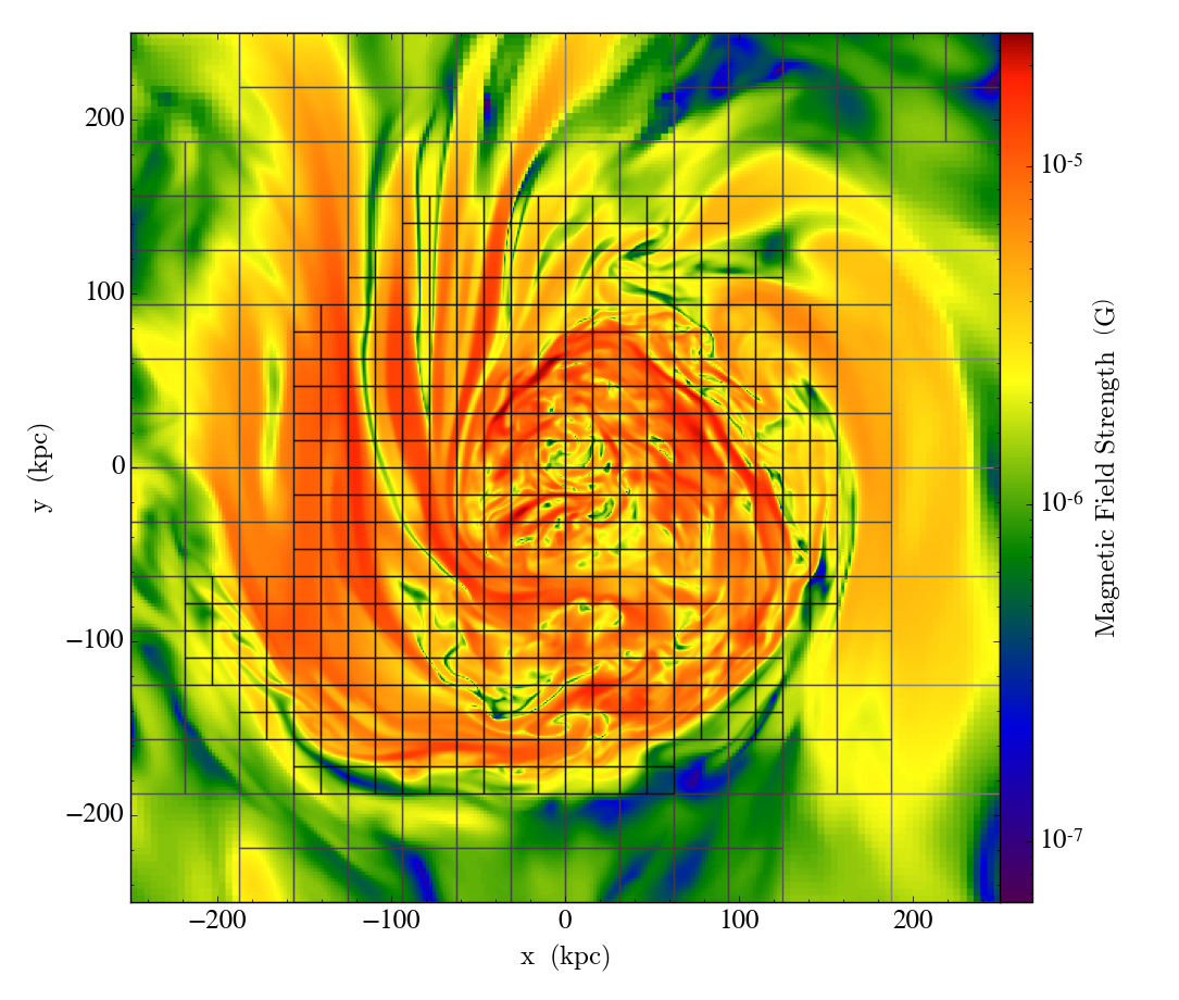
ds2 = yt.load('data/virgo_novisc.0054.gdf')
slc2 = SlicePlot(ds2, 'z', ['magnetic_field_strength'],
width=(500, 'kpc'), center='c')
slc2.show()

slc.set_cmap('density', 'magma')

Plot callbacks
slc.annotate_grids()

slc2.annotate_magnetic_field()

slc2.annotate_clear()
slc2.annotate_streamlines('velocity_x', 'velocity_y')

Line integral convolution (talk to Suoqing Ji, who is here!)
slc2.annotate_clear()
slc2.annotate_line_integral_convolution('magnetic_field_x', 'magnetic_field_y')

slc.save('my_amazing_plot.eps')
slc.save('my_amazing_plot.png')
from yt.units import mp
import numpy as np
def _sound_speed(field, data):
return np.sqrt(5./3.*data['kT']/(0.6*mp))
def _mach_number(field, data):
return data["velocity_magnitude"]/data["speed_of_sound"]
ds2.add_field(('gas', 'speed_of_sound'), _sound_speed, units='cm/s', force_override=True)
ds2.add_field(('gas', 'mach'), _mach_number, units='', force_override=True)
slc = yt.SlicePlot(ds2, 'z', ["speed_of_sound"], width=(200., 'kpc'))
slc.set_unit('speed_of_sound', 'km/s')
slc.set_log('speed_of_sound', False)
slc.set_zlim('speed_of_sound', 600., 1000.)

slc = yt.SlicePlot(ds2, 'z', ["mach"], width=(200., 'kpc'))
slc.set_log('mach', False)
slc.set_zlim('mach', 0.1, 0.8)

ProjectionPlot
from yt import ProjectionPlot
prj = ProjectionPlot(ds2, "z", 'density')
prj

prj.zoom(20)

prj.zoom(3)

ProjectionPlot(ds2, "z", 'density', width=(300.,"kpc"))

ProjectionPlot(ds2, "x", 'density', width=(300.,"kpc"))

ProjectionPlot(ds2, "y", 'density', width=(300.,"kpc"))

sp = ds.sphere("max", (5.0, 'Mpc'))
prj = ProjectionPlot(ds, "z", 'density', data_source=sp)
prj

ProjectionPlot(ds2, 2, 'kT', weight_field='density', width=(500, 'kpc'))

ProjectionPlot(ds2, 'z', 'density', width=(500, 'kpc'), method='mip')

Back to NumPy-like syntax
slc = ds.r[0.5,:,:] # slicing through the middle of the domain
p = slc.plot("density")

Back to NumPy-like syntax
d_m = ds.r[:,0.25:0.75,0.25:0.75].integrate('density', axis='x')
p_d = d_m.plot()

Back to NumPy-like syntax
kT_m = ds.r[:,0.25:0.75,0.25:0.75].mean("kT", axis="x", weight="density")
p_kT = kT_m.plot()

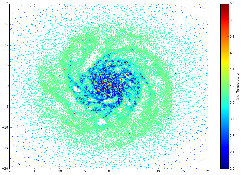
ParticleProjectionPlot
from yt import ParticleProjectionPlot
p = ParticleProjectionPlot(ds, "x", ("io","particle_mass"))
p.set_unit(('io', 'particle_mass'), 'Msun')

p = ProjectionPlot(ds, "x", ("deposit","all_density"))
p.show()

PhasePlot and ProfilePlot
from yt import PhasePlot
PhasePlot(ds.all_data(), 'density', 'temperature', 'cell_mass',
weight_field=None, fractional=True)

Analysis
- Profiles
- Fixed resolution buffers
- Covering grids
- Many more things that I don't have time to talk about in detail
Profiles
Profiles can create a 1D, 2D, or 3D histogram of a field versus a set of other fields.
We already saw a 2D histogram above when we made a PhasePlot of density, temperature, and cell mass
We can use profiles to calculate the average value or total of a field vs another field.
from yt import create_profile
sph = ds2.sphere(ds2.domain_center, (300., 'kpc'))
profile = create_profile(sph, ('radius'), ('density'), logs={'radius': False})
%matplotlib inline
import matplotlib
matplotlib.rc("font", size=18)
from matplotlib import pyplot as plt
plt.figure(figsize=(8,8))
plt.loglog(profile.x.to('kpc'), profile['density'].in_units('Msun/kpc**3'))
plt.xlabel('Radius (kpc)')
plt.ylabel(r'$\mathrm{\rho\ (M_\odot kpc^{-3})}$')

Fixed Resolution Buffer
Fixed resolution buffers are a uniform resolution 2D representation of a slice or a projection.
slc = ds.slice("z", 0.25)
frb = slc.to_frb((40.0,"Mpc"), 800)
plt.figure(figsize=(8,8))
plt.imshow(frb["velocity_magnitude"].v, origin='lower', interpolation='nearest')

Covering grids
Covering grids are a uniform resolution 3D representation of a yt dataset. Very useful for analysis tools that expect a uniform resolution grid, or for simplifying analysis to avoid thinking about AMR.
SlicePlot(ds2, "z", 'velocity_z', center='c', width=(0.1, "unitary"))

# create covering grid of z-velocity at AMR level 3
cgrid = ds2.covering_grid(3, left_edge=[-0.15, -0.15, -0.15], dims=[128, 128, 128])
velocity_field = cgrid["velocity_z"]
print (velocity_field.shape)
plt.figure(figsize=(8,8))
plt.imshow(velocity_field[:,:,70].T.v, interpolation='none', origin='lower')
plt.show()

Analysis Modules
IFrame("http://yt-project.org/docs/dev/analyzing/analysis_modules/index.html", width=700, height=600)
Volume Rendering
IFrame("http://yt-project.org/docs/dev/visualizing/volume_rendering.html", width=700, height=600)
What about...?
Q: What about Athena++?
A: Support for Athena++ is under development, and it mostly works. To get it now, come ask me after the talk or later this week. It will hopefully be merged into the main development branch soon.
What about...?
Q: What if I want to look at the data from the perspective of the way it's laid out on the mesh?
A: You can definitely do that. Each dataset has an index object that holds the mesh hierarchy:
print(ds.index.grids)
print(ds.index.grids[11].LeftEdge)
print(ds.index.grids[11].RightEdge)
print(ds.index.grids[11].ActiveDimensions)
print(ds.index.grids[11]['density'])
What about...?
Q: My favorite code doesn't appear to be supported. Can I still use yt?
A: Yes! For a start, we have ways of loading in generic array data:
load_uniform_gridUniformly gridded dataload_amr_gridsAMR dataload_particlesParticle dataload_hexahedral_meshSemi-structured mesh data
New Features in yt 3.3
- First-class support for unstructured meshes
- Improved volume rendering interface
- Interactive OpenGL volume rendering
- Easy conversions between different unit systems
- "NumPy-like" operations for data objects
Coming soon
- Improved support for non-cartesian geometries (spherical, cylindrical, PPV-cube, etc.)
- Improved scaling for datasets with particles
- Streamlining the process to get data into yt
Community
- Over 20,000 changesets since 2007 by over 100 unique contributors
- 350 subscribers to users mailing list, 120 subscribers to developer mailing list
- Funding for aspects of yt development comes from the NSF, NASA, and the Gordon and Betty Moore Foundation
Getting involved and asking for help
Documentation: http://yt-project.org/doc
Users mailing list: http://lists.spacepope.org/listinfo.cgi/yt-users-spacepope.org
Developer mailing list: http://lists.spacepope.org/listinfo.cgi/yt-dev-spacepope.org
Developer guide: http://yt-project.org/docs/dev/developing/index.html
Slack Channel: https://yt-project.slack.com
IRC Channel: http://yt-project.org/irc.html (or #yt on freenode with your favorite IRC client)